🏠 Back to the Table of Contents

Research results

Friction & wear

Sliding in frictional interfaces: stability and regularization

Being inspired by experiments [51] of Jay Fineberg’s group, in our early study [52] with David S. Kammer using velocity weakening friction law, we reproduced some experimental results, identified directionality effect and looked for an energetic criterion for slip propagation. At the same time, we questioned the validity of supersonic slip propagation which we observed in our numerical simulations (see double Mach cone in the animation below), for more discussion on this topic, the reader is referred to Section on supersonic slip pulses.

Show animation.

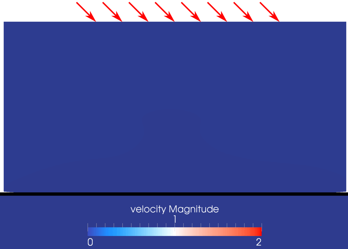
Animation demonstrating velocity of material points in a sheared and squeezed elastic block on a rigid substrate after spontaneous triggering of slip event. Velocity weakening friction law was used [52].

Finally, we discovered that the validity of the obtained results could demonstrate a strong dependence on the mesh density [53, 54, 55]. Therefore, we carried out a more fundamental study [56] on a deformable-rigid configuration using Prakash-Clifton regularization [57] for Coulomb’s friction law:
$$\dot\tau = - \frac{|v|+v_0}{L}(\tau - \mu p),$$
where $\tau$ is the limit frictional traction, $v$ is the slip velocity, $v_0$ is a reference velocity, $L$ is the characteristic regularization length, $\mu$ is the coefficient of friction and $p$ is the contact pressure assumed positive in contact. We studied the effect of the mesh density $h$ and regularization length $L$ on the convergence of slip events triggered by elliptic spatio-temporal pressure drop inspired from [55]. All triggered slip pulses eventually died.

The main result of this study are the following. We first confirmed that mesh-converged solutions are achievable in the stable regime (for friction coefficients smaller than one, see [58]) of the considered problem without any numerical damping in the bulk. We delimited a mesh-convergence map with respect to the characteristic length $L$ of the Prakash-Clifton friction law (see Fig. 18). This map confirmed that mesh-converged solutions for smaller lengths $L$ need finer mesh discretizations. In addition to the mesh convergence, we discovered a convergence of the solution with respect to the characteristic length $L$ itself. Considering a given slip event, a critical characteristic length $L_c$ exists, such that $\forall L: L < L_c$, the slip behavior of the interface remains the same. To confirm and explain this observation, we analyzed the regularization’s effect on a range of temporal frequencies of the frictional strength. The damping of low frequencies, which are the essential part of the slip event, becomes vanishingly small for small characteristic lengths and no longer influences the propagation of the interface rupture. This insight enables the definition of a theoretical domain $L > L_c$ of influence of the Prakash-Clifton friction law with respect to the characteristic length of the regularization and the frequency content of the slip event. Outside of this domain $L < L_c$, the damping of the slip event’s frequencies becomes negligible and the interface rupture propagates as if it was governed by Coulomb’s friction law despite the presence of the regularization. In conclusion, the presented results suggest that the experimental determination of the physical length scale $L_{\text{ph}}$ of the Prakash-Clifton friction law requires the temporal power spectrum density of the analyzed slip event to contain enough energy in the high-frequency domain. We therefore proposed a verification procedure for the slip event’s frequency content, which is crucial to a successful determination of $L_{\text{ph}}$, because if the propagation of slip is fully determined by frequencies below a critical value, the real physical length scale $L_{\text{ph}}$ of the Prakash-Clifton friction cannot be measured. The observed length scale instead would correspond to the critical length $L_c$, which could be significantly higher than the physical length scale $L_{\text{ph}}$.

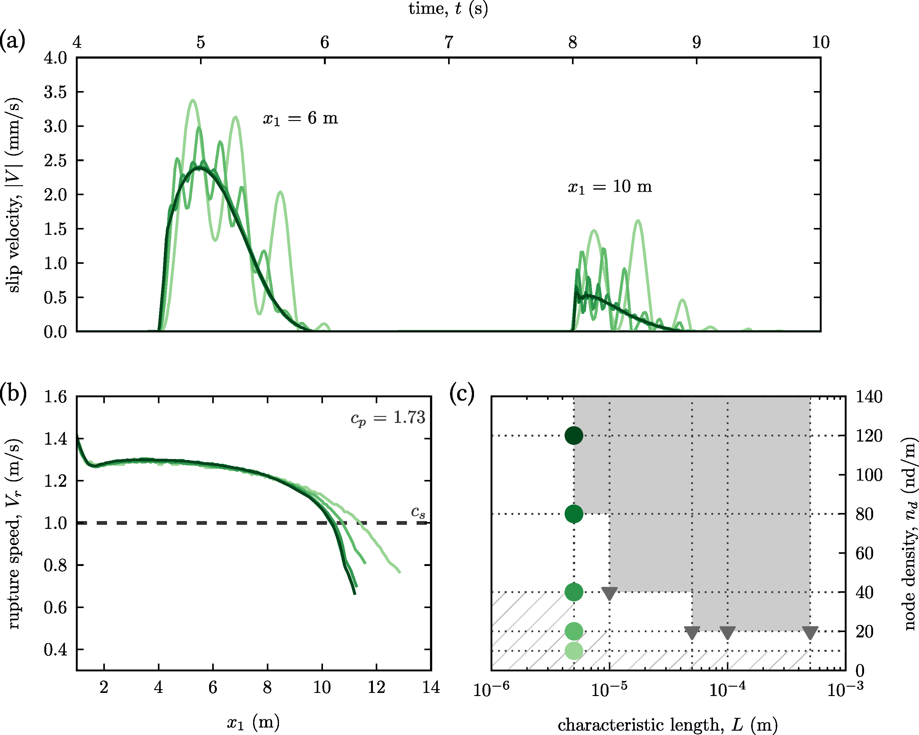
Illustration of mesh convergence for a frictional interface rupture with simplified Prakash-Clifton regularization $L = 5 \; \mu\text{m}$ and $v_0 = 100\; \mu\text{m/s}$. (a) The evolution of the slip velocity over time is shown at two positions. (b) The rupture speed change along the propagation distance $x_1$. © The convergence map in the $L - n_d$ plane ($n_d$ is the mesh density) indicates the zone of mesh-converged (gray area) whereas within the hatched area the results are considered to be non-converged. The circles designate the simulations presented in (a) and (b). The triangles mark mesh-converged simulations for different $L$.


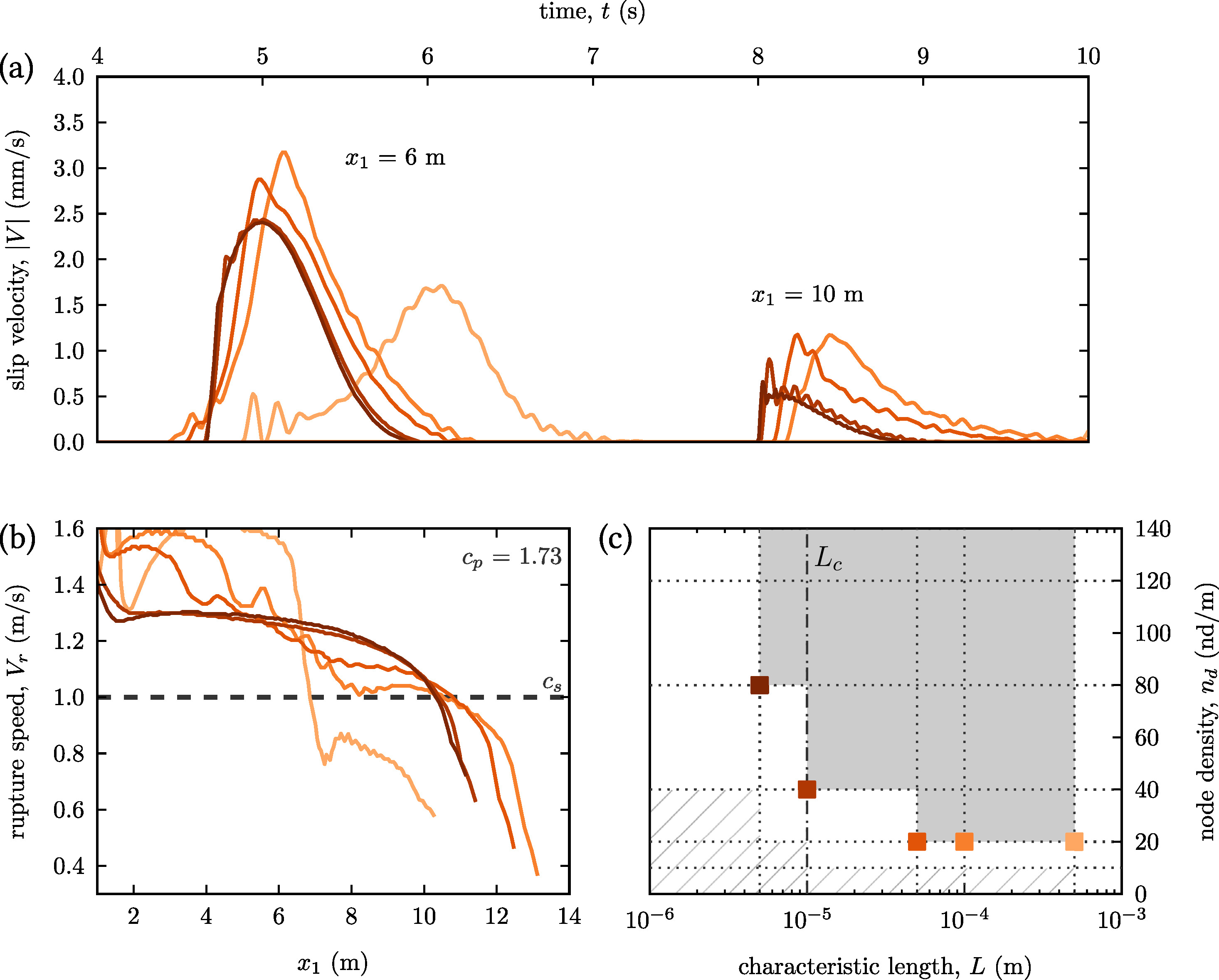
Fig. 18 The slip velocity in (a) and the rupture speed in (b) of mesh-converged simulations are shown for different characteristic lengths $L$. As one can see, both the morphology of the slip profile and the velocity of the slip front vary with the length $L$ however the further mesh refinement does not change these results. © The squares indicate the mesh density $n_d$ and characteristic length $L$ of the simulations presented in (a) and (b). All shown results are in the mesh-converged area of the $L - n_d$ plane. $L_c$ marks the critical characteristic length of the simplified Prakash-Clifton friction law for the presented interface rupture, below which all converged simulations have the same global and local behavior.

📚 References

• [52] D.S. Kammer, V.A. Yastrebov, P. Spijker, J.F. Molinari. “On the propagation of slip fronts at frictional interfaces”. Tribology Letters, 48(1):27-32 (2012). [doi] [arXiv] [pdf]
• [56] D.S. Kammer, V.A. Yastrebov, G. Anciaux, J.F. Molinari. “The existence of a critical length scale in regularised friction”. Journal of the Mechanics and Physics of Solids, 63:40-50 (2014). [doi] [arXiv] [pdf]

🏠 Back to the Table of Contents

---

Slip stability under non-uniform pressure distribution

A slip-weakening friction law can be seen as a simplified form of a generalized “rate and state” law. The former simplified form allows to make a direct link with the linear elastic fracture mechanics [59, 60, 61]. This analogy makes it possible to study the stability/instability of the sliding front propagation via the well-known fracture mechanics methods, i.e. by comparing the energy release rate $G$ with its critical value $G_c$. The energy release rate $G(x)$ of the frictional front depends on the external loading as well as on the residual stresses in the slip zone. As for $G_c$, it is proportional to the local contact pressure $G_c(x) \sim p(x)$. Until recently the studies focused on the uniform pressure, i.e. on the constant critical energy release rate, like in classical fracture mechanics, with some notable exceptions [62, 63]. In my recent study, under the "small scale yielding" (SSY) assumption [64], I managed to derive [65], under moderate and controllable assumptions, some fairly accurate results for two model pressure distributions (a) parabolic pressure profile:
$$\sigma(x) = \sigma_0 + \kappa x^2/2$$
and (b) localized pressure valley:
$$\sigma(x) = \sigma_0 + \begin{cases} \displaystyle8\Delta\sigma\left(\frac x \lambda\right)^2&,\text{ if }|x| \le \lambda/4\\[5pt] \displaystyle\Delta\sigma\left(\frac{8|x|}{\lambda}-\frac{8x^2}{\lambda^2}-1\right)&,\text{ if } \lambda/4 < |x| \le \lambda/2\\ \displaystyle\Delta\sigma &,\text{ if } |x| > \lambda/2.\\ \end{cases}$$
I have studied many slip scenarios in the case of an isolated valley (stable-instable, stable-instable-stable, etc.) for parameters relevant for geological faults (see Fig. 19).
Among other analytical results, I derived the minimum value of the pressure $\sigma_0$ needed to trigger the unstable slip for a given curvature:
$$\frac{\sigma_0}{\mu} > \left[\frac{3(f_s-f_k)^2 }{8\pi^2f_k }\cdot\frac{\kappa d_c^2}{(1-\nu)^2\mu}\cdot\frac{(2f_k+f_0)^2}{(f_0-f_k)^5}\right]^{1/3},$$
where $\mu$ is the shear modulus, $\nu$ is the Poisson’s ratio, $f_s,f_k$ are static and kinetic coefficients of friction, $d_c$ is the characteristic slip-weakening distance.
The arrest length for a parabolic valley was found to be:
$$a_s \approx 4\sqrt{\frac{\sigma_0(f_0-f_k)}{5\kappa f_k}} - \frac{ (f_s-f_k)d_c}{\pi(1-\nu)(f_0-f_k)^2}\cdot\frac{\mu}{\sigma_0},$$
I have also obtained an interesting result making a link between the macroscopic shear load rate $\dot \tau_0 = \sigma_0 \dot f_0$ and the crack-arrest rate $\dot a_s$:
$$\frac{\dot a_s}{\dot \tau_0} \approx \sqrt{\frac{4}{5\sigma_0\kappa f_k(f_0^0+\dot f_0 t)}} + \frac{2(f_s-f_k)d_c}{\pi(1-\nu)(f_0^0+\dot f_0 t)^3}\cdot\frac{\mu}{\sigma_0^2}$$
This equation allows to estimate the stable slip front advancement at geological scales as well as at the lab scales. For example, for the frictional experiments of Fineberg’s group [51], the stable crack advancement rate compared to the rigid loading rate is given by
$$\frac{\dot a_s}{\dot u} \approx 10^7\frac{1}{\sqrt{\kappa}} \left[\frac{\text{Pa}^{1/2}}{\text{m}^{1/2}}\right]$$
Suggesting that for small systems, even for a very slow loading $\dot u \ll c_s$, where $c_s$ is the transverse load speed, the local stable slip can be hardly distinguishable from a dynamic one and can be even supersonic. This result clearly explains the puzzling "slow slip events" obtained by the experimentators and also observed at geological scales [66, 51].

Version française (click to expand)

Une loi de frottement qui s’adoucit avec la distance de glissement peut être vue comme une forme simplifiée d’une loi de “rate and state” généralisée. L’avantage de la première est qu’un lien avec la mécanique linéaire de la rupture s’établit directement [59, 60, 61]. Cela permet donc d’étudier la stabilité/instabilité de la propagation du front de glissement via des méthodes établies de la mécanique de la rupture en comparant le taux de la restitution d’énergie $G$ avec sa valeur critique $G_c$. Le taux de restitution d’énergie $G(x)$ dépend du chargement externe ainsi que des contraintes résiduelles dans la zone de glissement. Quant à $G_c$, il est proportionnel à la pression de contact locale $G_c(x) \sim p(x)$. Jusqu’à récemment les seuls cas étudiés sont à pression uniforme, avec quelques exceptions notables [62, 63]. Dans mon étude récente, sous l’hypothèse de SSY [64] ("small scale yielding") j’ai réussi à dériver quelques résultats assez précis pour (1) la longueur de déstabilisation et (2) la distance d’arrêt de glissement, pour une distribution de pression (a) parabolique et (b) du type vallée isolée de pression (cf. Fig. 19). En outre, j’ai étudié de nombreux scénarios de glissement dans le cas d’une vallée isolée (stable-instable, stable-instable-stable, etc) et j’ai déduit la valeur minimale de pression $\sigma_0$ nécessaire pour déclencher le glissement instable :
$$\frac{\sigma_0}{\mu} > \left[\frac{3(f_s-f_k)^2 }{8\pi^2f_k }\cdot\frac{\kappa d_c^2}{(1-\nu)^2\mu}\cdot\frac{(2f_k+f_0)^2}{(f_0-f_k)^5}\right]^{1/3}.$$
Tous ces résultats font le lien entre plusieurs paramètres de frottement (coefficients statique $f_s$ et dynamique $f_k$, longueur caractéristique d’adoucissement $d_c$), la distribution de pression (valeur minimale $\sigma_0$, largeur de la vallée $\lambda$, courbure $\kappa$), et l’élasticité des corps (module de cisaillement $\mu$).
Ces résultats sont intéressants pour la physique des séismes car ils permettent d’analyser des scénarios de glissement dans des failles avec une hypothèse de distribution de pression plus élaborée que celle qui était considérée jusqu’à présent.
En outre, mes résultats suggèrent une nouvelle interprétation des "slow slip" découverts par l’équipe de Fineberg [67, 51].
La finalisation de l’article cité ci-dessous nécessite encore quelques calculs analytiques qui n’ont pas encore été achevés.

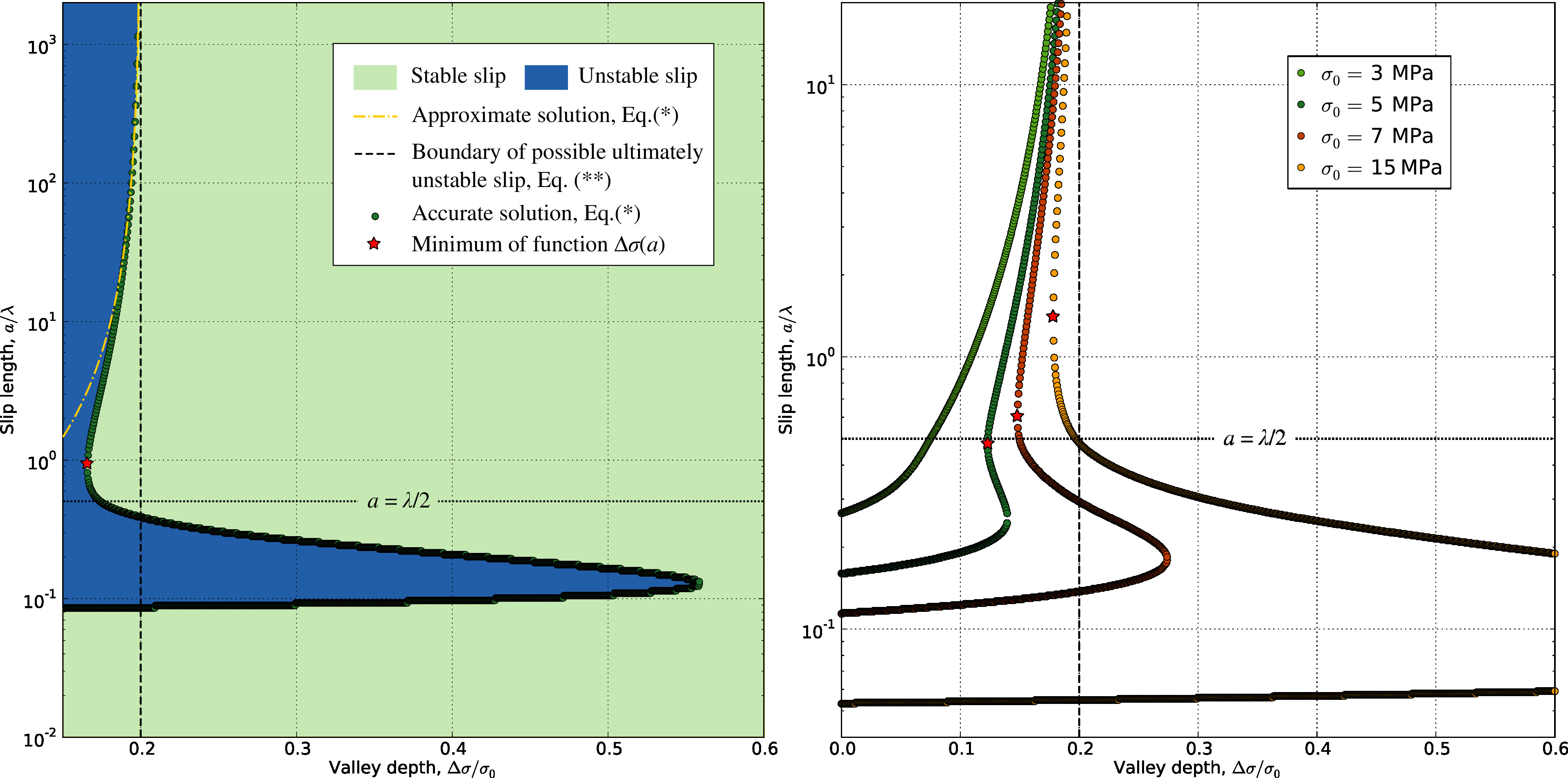Fig. 19

Slip stability map in the contact interface with a pressure valley located in the $\lambda$ interval of depth $\Delta\sigma$ for different valley pressures $\sigma_0$. The blue and green zones determine possible slip lengths in unstable and stable regimes, respectively.

Version française (click to expand)

Carte de stabilité du glissement dans l’interface de contact avec une vallée de pression localisée dans l’intervalle $\lambda$ de profondeur $\Delta\sigma$ et de pression minimale $\sigma_0$. Les zones bleue et verte déterminent des longueurs de glissement possible dans des régimes instables et stables respectivement.

📚 References

• [65] Yastrebov, VA. “Slip propagation along slip-weakening interfaces with a non-uniform contact pressure distribution” (2021). Draft is available [encrypted pdf]
• Presentation “Slip propagation at interfaces with a non-uniform contact pressure distribution”, CECAM Workshop “Modeling tribology: friction and fracture across scales”. Lausanne, Switzerland. January 29, 2019 [pdf]

🏠 Back to the Table of Contents

---

Opening waves: sliding without slipping

In a theoretical study that combines analytical calculations and dynamic finite element simulations with implicit integration, I explored the complex phenomenon of sliding of an elastic layer ($E,\nu,rho$) of height $H$ on a rigid substrate with an interface governed by a Coulomb’s friction law with a friction coefficient $f$. In finite systems, the elasto-dynamic slip under the action of frictional forces is strongly coupled to the propagation of elastic waves in the system which serves as a wave-guide and ensures their dispersive propagation [68]. By reducing the infinite system to a periodic system with period $L$, and introducing the notation $r = H/L$ the uniform sliding stability can be determined by solving the transcendental equation:
$$\begin{split} & f \left[\sin(2\pi\kappa_d K r)+\kappa_s\kappa_d\sin(2\pi\kappa_s K r)\right]\left(-2\kappa_d\kappa_s\sin(2\pi\kappa_d K r) + (\xi^2+\gamma^2\kappa_d^2)\sin(2\pi\kappa_s K r)\right)-\\ &-f\kappa_s\kappa_d\left[\cos(2\pi\kappa_d K r) -\cos(2\pi\kappa_s K r)\right]\left(2 \cos(2\pi\kappa_d K r) + (\xi^2+\gamma^2\kappa_d^2)\cos(2\pi\kappa_s K r)\right)+\\ &+i\kappa_d\left[2+\xi^2(\kappa_s^2-1)\right]\left( \cos(2\pi\kappa_d K r) \sin(2\pi\kappa_s K r) + \kappa_s\kappa_d\cos(2\pi\kappa_s K r)\sin(2\pi\kappa_d K r)\right) = 0 \end{split} (\#eq:transc)$$
with
$$\kappa_d = \sqrt{k_d^2/k^2 - 1},\quad \kappa_s = \sqrt{k_s^2/k^2 - 1},\quad k = 2\pi K / L, \quad \xi = \frac{2\nu}{(1-2\nu)}, \quad \gamma = \sqrt{\frac{2(1-\nu)}{1-2\nu}},$$
The numerical solution of this equation shows that uniform sliding in a finite size system is always unstable, but it also predicts the velocity of stick-slip fronts that form due to this instability, which compares well with the numerical results. Numerically, we have also shown that the macroscopic friction depends on the imposed slip velocity, even if locally the Coulomb friction law does not depend on the velocity! This interesting result confirms the analytical calculation of G.G. Adams [69] by transposing it to finite size systems. This theoretical part has not been published yet, but I hope to restart this work very soon.

When the friction coefficient is very high (above $1$), the sliding regime differs greatly from the local stick-slip regime. It is distinguished by the emergence of opening waves that allow macroscopic sliding almost without friction [70], a theoretical phenomenon that attracted a particular attention of the fracture mechanics community at some point [71, 72, 73] but, as it seems to me, was forgot for a while. On the other hand, these opening waves are different from Schallamach waves and they propagate at intersonic speeds in the interface. In this scenario the released elastic energy transforms almost entirely into elastic waves and allows the body to "jump" into a deformed configuration that is antisymmetric with respect to the sliding onset configuration to adhere again. This "jump" reverses the direction of the frictional force which thus becomes macroscopically "negative" (!) (cf. Fig. 20). These unusual results, which echo other theoretical results [74, 75], await their experimental verification. The confirmation of this process will allow the optimization of friction-based systems and better understanding of slip dynamics.

Version française (click to expand)

Dans une étude théorique qui combine des calculs analytiques et des simulations par éléments finis dynamique avec l’intégration implicite, j’explore le phénomène complexe de glissement d’une couche élastique ($E,\nu,rho$) de hauteur $H$ sur un substrat rigide avec une interface gouvernée par une loi de Coulomb avec un coefficient de frottement $f$. Dans des systèmes de taille finie, le glissement élasto-dynamique sous l’action des efforts de frottement est fortement couplé à la propagation des ondes élastiques dans le système qui sert de guide d’ondes et assure la propagation dispersive [68]. En réduisant le système infini à un système périodique avec une période $L$, et en introduisant la notation $r = H/L$ la stabilité de glissement uniforme peut être déterminée en résolvant l’équation transcendante :
$$\begin{split} & f \left[\sin(2\pi\kappa_d K r)+\kappa_s\kappa_d\sin(2\pi\kappa_s K r)\right]\left(-2\kappa_d\kappa_s\sin(2\pi\kappa_d K r) + (\xi^2+\gamma^2\kappa_d^2)\sin(2\pi\kappa_s K r)\right)-\\ &-f\kappa_s\kappa_d\left[\cos(2\pi\kappa_d K r) -\cos(2\pi\kappa_s K r)\right]\left(2 \cos(2\pi\kappa_d K r) + (\xi^2+\gamma^2\kappa_d^2)\cos(2\pi\kappa_s K r)\right)+\\ &+i\kappa_d\left[2+\xi^2(\kappa_s^2-1)\right]\left( \cos(2\pi\kappa_d K r) \sin(2\pi\kappa_s K r) + \kappa_s\kappa_d\cos(2\pi\kappa_s K r)\sin(2\pi\kappa_d K r)\right) = 0 \end{split} (\#eq:transc)$$
avec
$$\kappa_d = \sqrt{k_d^2/k^2 - 1},\quad \kappa_s = \sqrt{k_s^2/k^2 - 1},\quad k = 2\pi K / L, \quad \xi = \frac{2\nu}{(1-2\nu)}, \quad \gamma = \sqrt{\frac{2(1-\nu)}{1-2\nu}},$$
La résolution numérique de cette équation montre que le glissement uniforme dans un système de taille finie est toujours instable, mais elle prédit également la vitesse des fronts de "stick-slip" qui se forment à cause de cette instabilité, qui se compare bien avec les résultats numériques. Numériquement, nous avons également montré que le frottement macroscopique dépend de la vitesse de glissement imposée, même si localement la loi de frottement de Coulomb ne dépend pas de la vitesse ! Ce résultat intéressant confirme le calcul analytique de G.G. Adams [69] en le transposant aux systèmes de taille finie. Cette partie théorique n’a pas encore été publiée, mais j’espère poursuivre ce travail très bientôt.

Quand le coefficient de frottement est très élevé, le régime de glissement diffère beaucoup du régime de stick-slip habituel. Il se distingue par l’émergence d’ondes d’ouverture qui permettent de glisser macroscopiquement presque sans frotter [70]. Par contre, ces ondes d’ouverture sont différentes des ondes de Schallamach et elles se propagent à des vitesses intersoniques dans l’interface. Dans ce scénario l’énergie élastique libérée se reporte presque entièrement dans les ondes élastiques et permet au corps de “sauter” dans une configuration déformée antisymétrique par rapport à la configuration du début de glissement pour y adhérer de nouveau. Ce “saut” inverse la direction de la force de frottement qui devient donc macroscopiquement “négative” (cf. Fig. 20). Ces résultats insolites, qui font écho avec d’autres résultats théoriques [74, 75], attendent leur vérification expérimentale. La confirmation de ce processus permettra d’optimiser des systèmes basés sur le frottement, par exemple des freins.

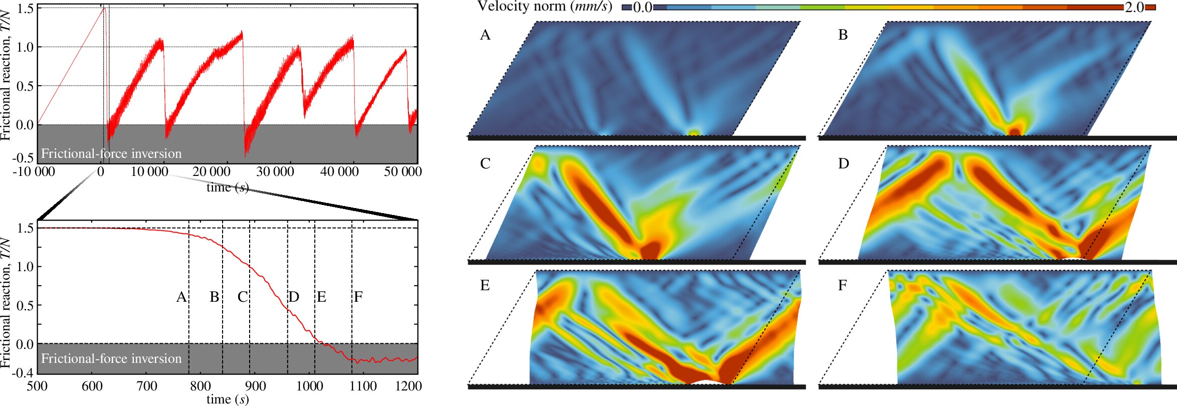Fig. 20 Inversion of the frictional force with time and emergence of opening waves in the interface (displacements are magnified by a factor of 150).

Version française (click to expand)

Changement de signe de la force de frottement au cours du temps et émergence des ondes d’ouverture dans l’interface (les déplacements sont multipliés par un facteur 150).

📚 References

• [70] V.A. Yastrebov. “Sliding without slipping under Coulomb friction: opening waves and inversion of frictional force”. Tribology Letters, 62(1):1-8 (2016) [doi] [arXiv] [pdf]
• V.A. Yastrebov “Elastodynamic Friction” presentation from the course “Contact Mechanics and Elements of Tribology” (seminar lecture) [pdf]

🏠 Back to the Table of Contents

---

Supersonic slip pulses in Coulomb’s driven frictional interfaces

In his brilliant paper G.G. Adams [69] studied the possibility of radiation of bulk waves by an isolated slip pulse propagating under classical Coulomb’s friction law at the interface between an elastic half-plane and a rigid plane. Naturally, the trace speed of these bulk waves in the interface are supersonic, i.e. the slip front propagates as supersonic velocity $c>c_p$. This result causes questions on the causality of such theorized events. This interesting result inspired our interest and with David S. Kammer, and since recently with his group at ETHZ, we started to study numerically the possibility to initiate self-sustained supersonic slip pulses in such frictional interfaces. In reality, the slip velocity of such pulses is only marginally higher than the longitutidal wave speed $c_p$ and strongly depends on the Poisson’s ratio $\nu$, the directionality of the triggering event, and the whole system dynamics is strongly affected by the proximity of the stress state in the interface to the frictional limit $0 \le |\tau|/(\mu p) < 1$. Currently, apart from the theoretical study of related slip pulses, we could demonstrate that in some scenarios the slip propagation is unstable regardless the fact of being in theoretically stable regime for a uniform slip ($\mu < 1$, see [58]), the Prakash-Clifton regularization slows down the frictional pulses thus preventing from obtaining a mesh converged and supersonic pulses at the same time. Nevertheless, some numerical results for particular configurations make us hope that supersonic slip pulses in semi-infinite systems can exist in absence of wave-guide modes and without the influence of reflected waves hitting the interface. The work continues.

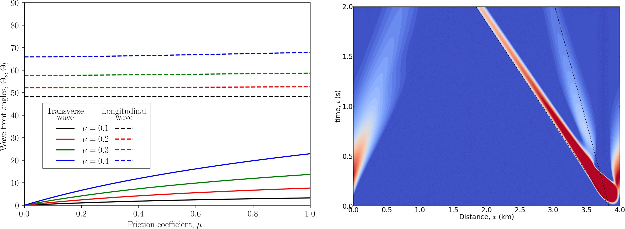
(left) – Adams’ solution for the inclination angle of radiated bulk waves demonstrating that their trace speed increases with the coefficient of friction and with the Poisson’s ratio, (right) – simulation results (for periodic BC) for supersonic triggering event demonstrating an emerging self-sustained slip pulse propagating at the longitudinal wave speed in the direction opposite to the shear direction ($\mu=0.2$, $\nu=0.4$), still it is not a supersonic pulse.

🏠 Back to the Table of Contents

---

Multiscale simulation of hardmetal interaction with rocks

In the framework of NEXT-DRILL project, with Georges Cailletaud, Charlie C. Li and Alexandre Kane we supervised PhD project of Dmitry Tkalich. The origin of the wear of hardmetal inserts in rotary-percussive hard-rock drilling is a puzzling phenomenon. We suspect that this wear cannot be explained by abrasive interaction with rock debris, but rather by a friction-induced tensile stress state on the leading edge of hardmetal insert during the oblique impacts of the rock [76]. We carried out multi-scale finite element simulation including (see Fig. 21):

• accurate full-field microstructural representation of the hardmetal (WC/binder) for different volume fraction of the binder,
• calibration of the mean-field $\beta$-model [77] on various monotonic loadings of full-field microstructures with Drucker-Prager model for WC grains and $J2$ plasticity for the binder,
• full-scale simulation of a frictional oblique impact of a hardmetal insert using mean-field $\beta$-model at every Gauss point of the insert and an elastic rock Behavior,
• loading trajectory recovered in full-scale simulations are applied on the microstructural scale to reveal the underlying deformation and “damage” mechanisms.

This study demonstrated strong “plastic deformation” of WC grains near the leading of drilling inserts impacting the rock, which in the real life context would imply cracking and subsequent elimination of WC grains, which being ejected in the contact interface can cause more damage in intimate rock-tool contacts.

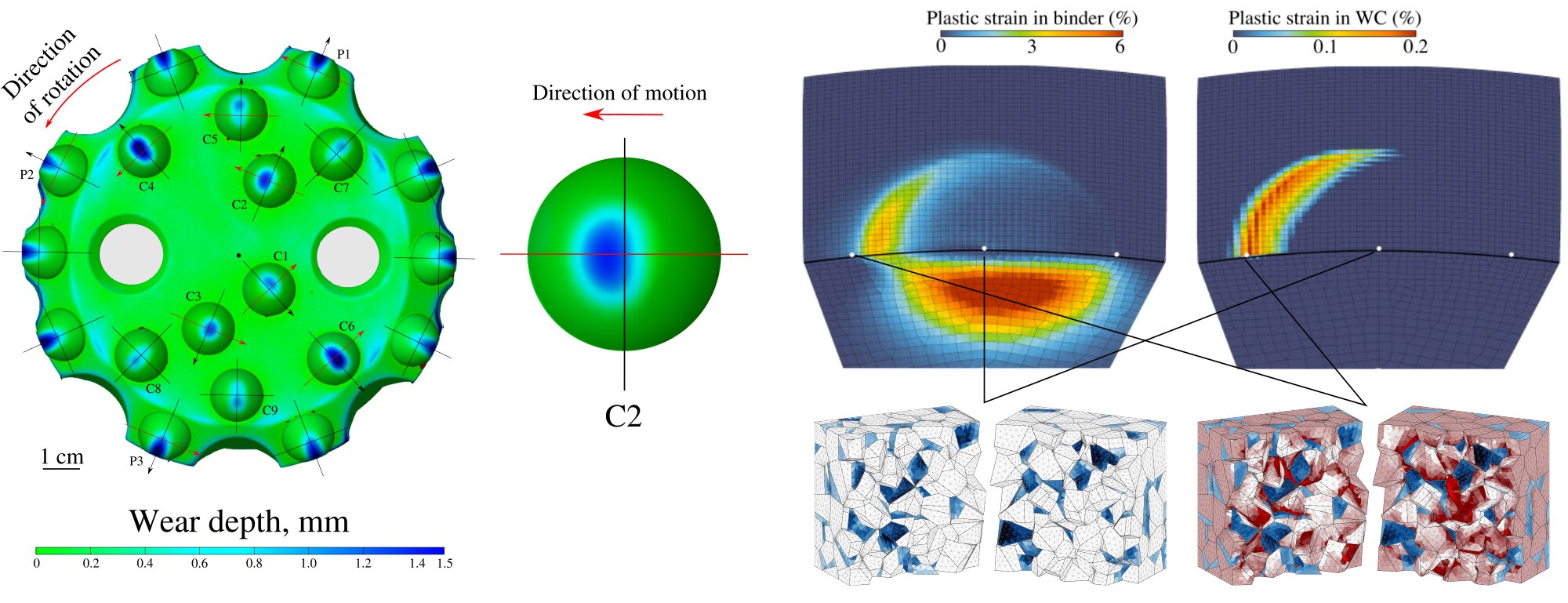Fig. 21

Wear pattern on percussive-rotary drill crown and hardmetal (WC/Co) inserts after drilling 80 m in hard rock formations. The asymmetry of the wear pattern is highlighted. On the right – accumulated plastic slip in WC and the binder, obtained in structural impact simulations using the calibrated mean-field model, below we show the results of accumulated plastic deformation on the microstructural level for the leading edge and central locations obtained using the full-field FE model after simulating the full loading cycle $\boldsymbol\sigma(t)$ coming from the macro-scale simulation: blue - plasticity in the binder, red - plasticity in WC grains.

In addition, within the same study we studied small scale damage and plasticity of hardmetal composites in interaction of hard fractions of hard-rocks, both plastic deformation and interface debonding were included in the full model.

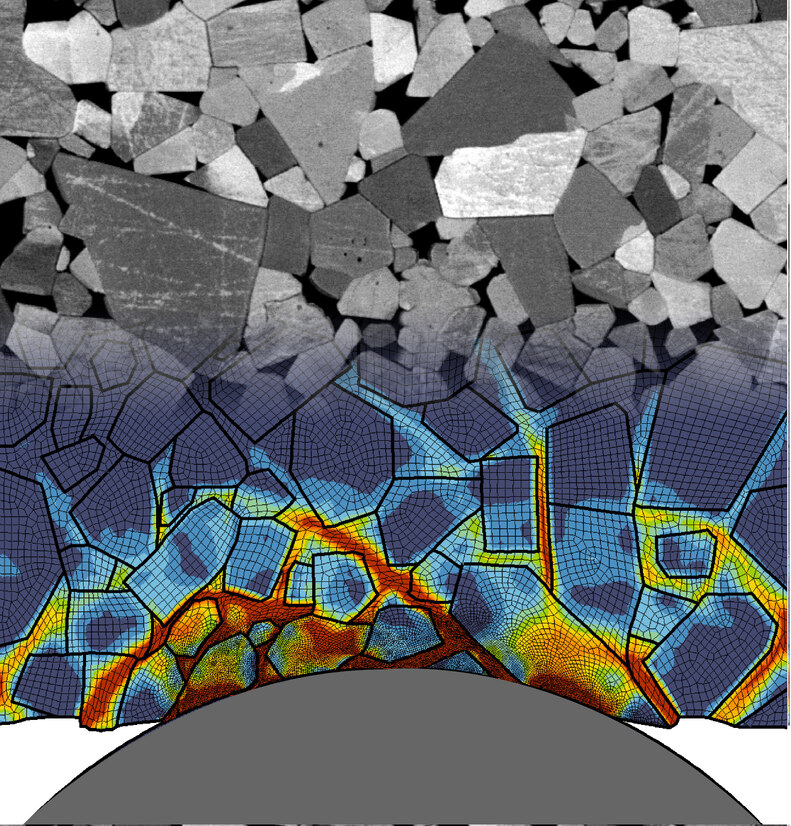
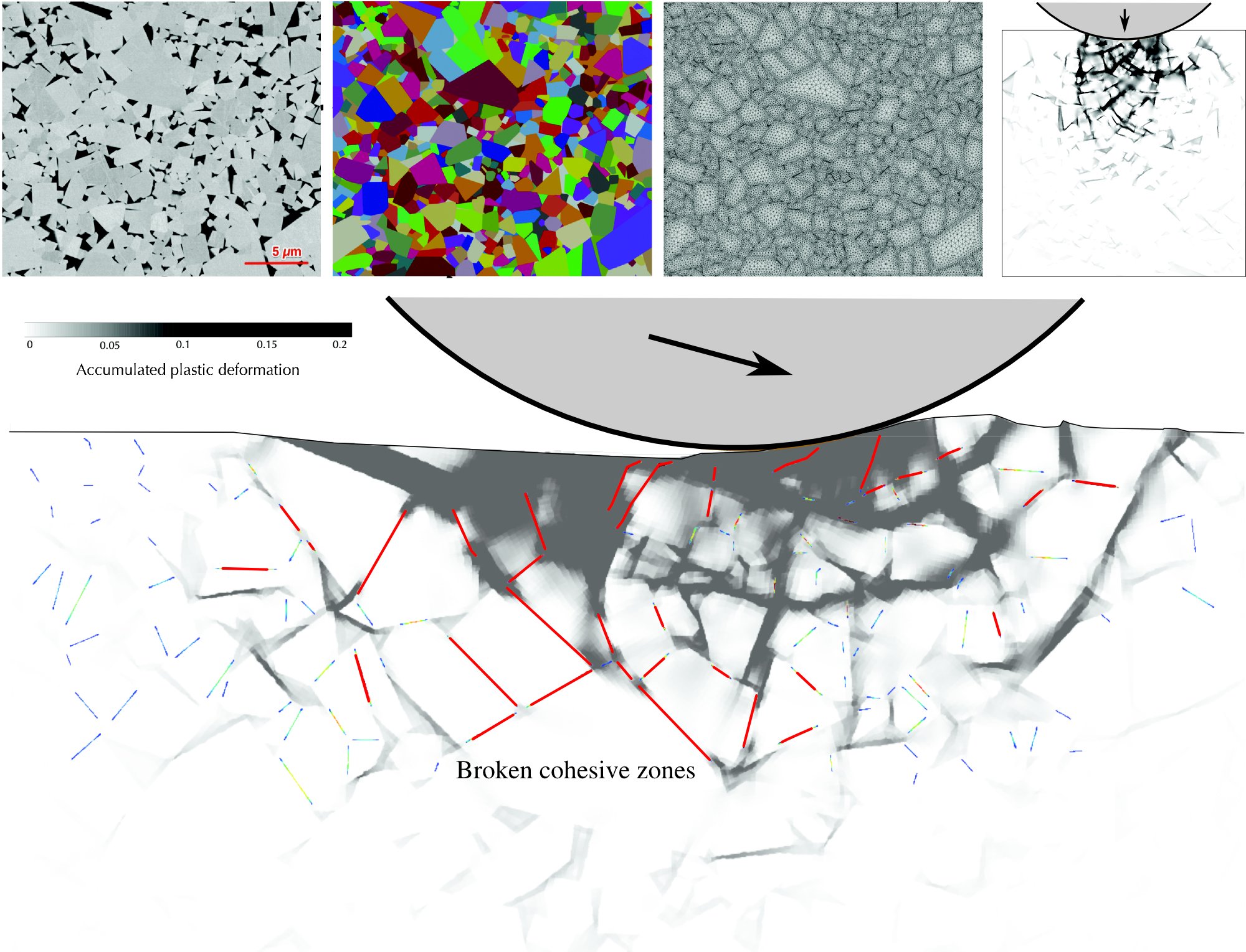
Left – Simulation of an impact of a hardmetal microstructure by a rigid indenter representing a smooth hard fraction of the rock, plastic deformations in the binder and WC grains is shown, in the background the true SEM image of the microstructure is shown. Right – construction procedure of plane WC/Co microstructure directly from SEM image and associated simulations of the normal and oblique impacts, red lines show fully debonded WC/Co and WC/WC interfaces.

📚 References

• [78] D. Tkalich, A. Kane, A. Saai, V.A. Yastrebov, M. Hokka, V.T. Kuokkala, M. Bengtsson, A. From, C. Oelgardt, Ch. C. Li. “Wear of cemented tungsten carbide percussive drill-bit inserts: laboratory and field study”. Wear, 386:106-117 (2017). [doi] [pdf]
• [76] D. Tkalich, V.A. Yastrebov, G. Cailletaud, A. Kane. “Multiscale Modeling of Cemented Tungsten Carbide in Hard Rock Drilling”. International Journal of Solids and Structures, 128:282-295 (2017). [doi] [pdf]
• Presentation “Multiscale wear modelling of cemented tungsten carbide tools in hard rock drilling” given at the conference “Computational Modeling of Complex Materials Across the Scales”, Nov 8, 2017. Paris, France [pdf]

🏠 Back to the Table of Contents

---

Pressure-dependent friction

According to the adhesive theory of friction, the maximum tangential force that the friction interface can undergo without sliding results simply from the product of the tangential resistance $\tau_c$ by the contact area $A$; as the contact area evolves in a first approximation linearly with the pressure $p_0$ applied to the apparent area $A_0$, the maximum friction force can be described as $T= \tau_c A \sim \tau_c p_0 A_0 \sim \tau_c N$, $N$ being the normal force. This provides the explanation of the Coulomb friction model. But if one improves the model describing the evolution of the contact area with the pressure, one can find a finer law [18] which takes into account the dependency on the pressure. Thanks to these results, it is straightforward to obtain the following pressure-dependent expression for the coefficient of friction:
$$\mu (p_0) = \mu_0 \left(1 - \frac{g (\alpha)}{\sqrt{2m_2}} \cdot \frac{p_0}{E^*}\right) \quad \text{ with } \quad \mu_0 = \frac{f(\alpha)\tau_c}{E^*\sqrt {2m_2}} (\#eq:pres_dep_fric)$$
where the $f(\alpha), g (\alpha)$ are universal functions of the Nayak parameter which have been determined numerically in [18], and $E^*$ is the effective elastic modulus of the interface.
Of course, this dependence remains phenomenological, but it nevertheless makes the link between the evolution of the pressure and the characteristics of the surface such as $m_2$ and $\alpha$, as well as with the elastic constants of the materials in contact $\nu_i, E_i$ which are contained in $E^*$. This law remains valid for linearly elastic materials and up to approximately $15$ % of the contact area.

In another study of contact in presence of a strongly non-compressible fluid trapped in the contact zone [30], we were able to demonstrate via simulations that the static frictional limit $\max(F_t)$ can behave like a non-monotonic function reaching its maximum and decreasing for very high pressures $p$, i.e. the friction can decrease while the pressure increases:
$$\frac{\partial \max(F_t)}{\partial | p |} < 0.$$
The friction can vanish completely for a critical pressure! The curve of the evolution of static friction with pressure Fig. 22 looks like the Drucker-Prager (or Mohr-Coulomb) law with a cap, which describes, among other materials, the behavior of rocks containing a multitude of pressurized cracks in the presence of fluid. This similarity to some extent confirms the validity of this rather exotic result of the decreasing friction.

Version française (click to expand)

Selon la théorie adhésive du frottement, la force maximale tangentielle que l’interface frottant peut subir sans glissement résulte simplement du produit de la résistance tangentielle $\tau_c$ par l’aire de contact $A$ ; comme l’aire de contact évolue en première approximation linéairement avec la pression $p_0$ appliquée sur l’aire apparente $A_0$, la force de frottement maximale peut être décrite comme $T = \tau_c A \sim \tau_c p_0 A_0 \sim \tau_c N$, $N$ étant la force normale. Ceci fournit l’explication du modèle de frottement de Coulomb. Mais si l’on améliore le modèle décrivant l’évolution de l’aire de contact avec la pression, on peut trouver une loi plus fine\cite{yastrebov2017jmps} qui prend en compte la dépendance à la pression. Grâce aux résultats obtenus en\cite{yastrebov2017jmps}, il est très facile d’obtenir le coefficient de frottement suivant :
ParseError: KaTeX parse error: Undefined control sequence: \label at position 162: …*\sqrt{2m_2}} \̲l̲a̲b̲e̲l̲{eq:fric}
où les $f(\alpha),g(\alpha)$ sont des fonctions universelles du paramètre de Nayak qui ont été déterminées numériquement dans [18], et $E^*$ est le module élastique effectif de l’interface.
Bien entendu, cette dépendance reste phénoménologique, mais elle fait néanmoins le lien entre l’évolution de la pression et les caractéristiques de la surface telles que $m_2$ et $\alpha$, ainsi qu’avec les constantes élastiques des matériaux en contact $\nu_i,E_i$ qui sont contenues dans $E^*$. Cette loi reste valide jusqu’à approximativement $15$ % de l’aire de contact.

Dans une autre étude du contact en présence d’un fluide fortement non-compressible piégé dans les zones de contact [30], nous avons pu démontré par des simulations que la limite de frottement statique $\max(F_t)$ peut se comporter comme une fonction non-monotone et pour des pressions très élevée $p$, diminue avec la pression croissante:
$$\frac{\partial \max(F_t)}{\partial |p|} < 0,$$
qui pour une pression critique peut rendre le frottement statique nulle ! La courbe de l’évolution du frottement statique avec la pression Fig. 22 fait penser à la loi de Drucker-Prager (or Mohr-Coulomb) avec "un cap" décrivant, entre autres, le comportement des roches comportant une multitude de fissures en contact et en présence de fluide. Cette similitude est une confirmation même si partielle et implicite de la validité de ce résultat exotique sur le frottement decroissant avec la pression.

Fig. 22(a) The evolution of the static friction as a function of the applied pressure $p/E^*$, the curve is non-monotonic and looks like a Drucker-Prager model with a "cap", the von Mises stress state in the wavy profile (only a half is shown) brought in contact with a rigid flat in presence of the non-saturated incompressible fluid in the interface (b) at low pressure and (c) at the moment when the fluid opens the trap and occupies the entire contact interface (the red area shows the size of the contact).

Version française (click to expand)

(a) L’évolution du frottement statique en fonction de la pression appluquée, la courbe est non-monotone et ressemble au comportement du modèle de Drucker-Prager avec un “cap”, l’état de contrainte de von Mises (b) peu après la mise en contact et (c) à l’ouverture du contact par le fluide qui s’échape du piége (la zone rouge démontre la taille du contact, juste une demi onde du profil sinusoïdale est montrée).

📚 References

• [18] V.A. Yastrebov, G. Anciaux, J.F. Molinari. “The role of the roughness spectral breadth in elastic contact of rough surfaces”. Journal of the Mechanics and Physics of Solids, 107:469-493 (2017) [doi] [arXiv] [pdf]
• [30] A.G. Shvarts, V.A. Yastrebov. “Trapped fluid in contact interface”. Journal of the Mechanics and Physics of Solids, 119:140-162 (2018). [doi] [arXiv] [pdf]

🏠 Back to the Table of Contents   ⏪ Previous page   ⏩ Next page