🏠 Back to the Table of Contents
Research results
Contact and multi-physics
Involved people:
 Andrei Shvarts (PhD, MINES 2016-2019, now at University of Glasgow),
 Guillaume Anciaux (EPFL),
 Georges Cailletaud (MINES ParisTech),
Jean-François Molinari (EPFL),
 Andreas Almqvist (Luleå University of Technology),
Francesc Pérez-Ràfols (PhD, Luleå University of Technology),
Paul Beguin (PhD student, MINES 2020-now),
Samuel Forest (MINES ParisTech),
 Vikram Phalke (PhD student, ITN),
Aurélien Fouque (PhD, MINES/CentraleSupélec 2016-2020, now at Siemens),
Frederick Sorel Mballa Mballa (postdoc, MINES/CentraleSupélec, 2013-2015, now at Vitrociset),
Julian Durand (PhD, MINES 2009-2012, now at Areva)
Contact mechanics at the roughness scale represents a holy grail of tribology providing a better understanding of contact, friction, wear, lubrication, sealing, as well as electrical and thermal conductivity at the system scale [1]. We have been working on this subject since the period of my PhD project, when in parallel with my own thesis, I participated in another doctoral study on the rough contact [2], which was like mine supervised by Georges Cailletaud. My contributions in this field focus on understanding the role of surface roughness in the process of deformation of elastic, elasto-plastic and viscoelastic bodies, as well as on the study of energy and mass transfers through and along contact interfaces. Emphasis is put on elastic contact for which analytical theories exist and which poses many important questions about the limits of surface fractality, the limits of continuous description and the relevance of various topographic parameters. This work requires efficient and precise numerical tools, a thorough statistical analysis, rather large parametric spaces and of course a sharp interpretation. All these elements have been implemented in our studies to draw relevant conclusions.
Version française (click to expand)
La mécanique du contact à l’échelle de la rugosité représente un Graal dans la compréhension du contact, du frottement, de l’usure, de la lubrification, de l’étanchéité, ainsi que de la conductivité électrique et thermique [1]. Je travaille sur ce sujet depuis la période de mon doctorat. C’est en effet dès cette époque que j’ai participé en parallèle de ma propre étude de thèse à une autre étude doctorale sur le sujet, qui était comme la mienne encadrée par mon directeur de thèse Georges Cailletaud. Mes contributions dans ce domaine se focalisent sur la compréhension du rôle de la rugosité dans le processus de déformation des corps élastiques, élasto-plastiques et viscoélastiques, ainsi que sur l’étude des transferts d’énergie et de masse à travers et le long des interfaces de contact. L’accent est mis sur le contact élastique pour lequel des théories analytiques existent et qui pose beaucoup de questions de fond sur les limites de la fractalité des surfaces, sur les limitations de la description continue et sur la pertinence de divers paramètres topographiques. Ce travail nécessite des outils numériques efficaces et précis, une analyse statistique poussée, des espaces paramétriques assez larges et bien entendu une interprétation pointue. Tous ces éléments ont été mis en œuvre dans mes (nos) études pour en tirer des conclusions pertinentes.
🏠 Back to the Table of Contents
Wavy surface in contact
We revisited the classic problem of an elastic solid with a two-dimensional wavy surface squeezed against an elastic flat half-space from infinitesimal to full contact [3]. Through extensive numerical calculations using the boundary and the finite element methods as well as using analytic derivations, we discover previously overlooked by Johnson, Greenwood and Higginson [3] transition regimes [4]. These transition (see Fig. 1) are seen in the evolution with applied load of the contact area and perimeter, in the mean pressure and in the probability density of contact pressure. They occur close to the percolation of initially separate contact-area spots. In addition, while studying this problem, I was interested by the geometrical characteristics of contact clusters, notably the so-called compactness which can be defined as the ratio of the square root of the area to the perimeter :
which is maximal for a circle and tends to zero for fractal forms for which the perimeter tends to for constant area. Finally, using famous differentiation under the integral sign (see Richard Feynman "Surely You’re Joking, Mr. Feynman!" Part 2. A different box of tools.), I could found an anlytical expression for the probability density of heights of a regular wavy surface , which turns to be
where
is the incomplete elliptic integral of the first kind. The singularity at is justified by saddle points.
Version française (click to expand)
Nous avons révisé le problème classique du contact normal entre une surface bi-sinusoïdale et un plan rigide. Numériquement nous avons pu démontrer [4] que la courbe maîtresse proposée par Johnson et al [3] n’est pas tout à fait correcte et qu’elle doit comporter un changement de signe de courbure près du point de percolation des zones de contact associées avec des crêtes différentes. Ce changement rapide provoque une décroissance de pression moyenne de contact même si l’aire de contact ainsi que la force continuent à augmenter (cf Fig. 1).
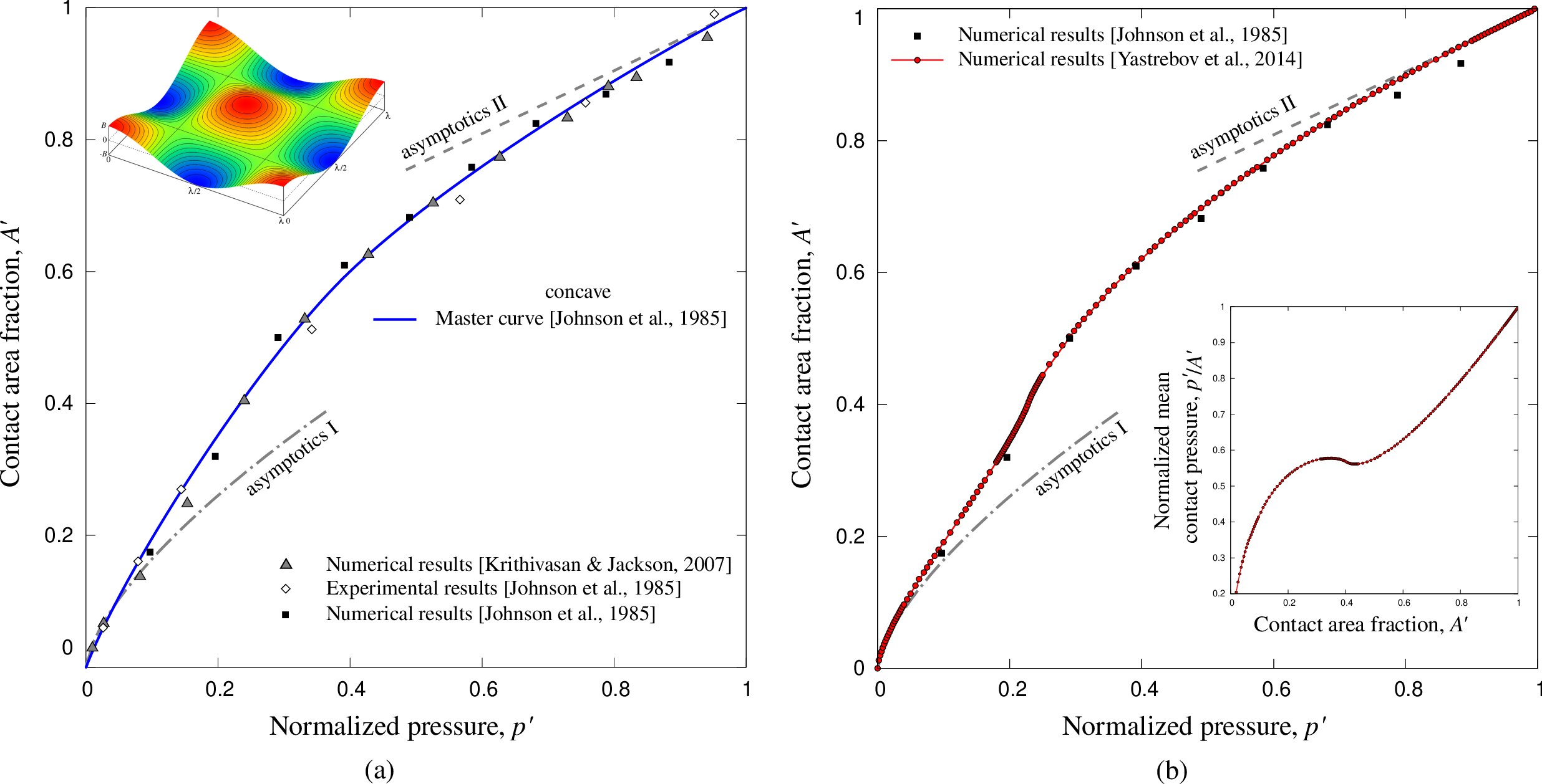 Fig. 1
Evolution of the contact area with the normalized pressure for a bi-sinusoidal surface brought in normal contact: (a) results from the literature where the transition was missed by the construction of a master curve [5, 3], (b) results of our simulations capturing the transition near percolation point, in the inset we show that the mean pressure can decrease even when the external pressure increases.
Version française (click to expand)
Évolution de l’aire de contact avec la pression normalisée d’une surface bi-sinusoïdale : (a) résultats de la littérature où une transition intéressante a été manqué par la construction d’une courbe maîtresse [5, 3], (b) notre solution numérique capturant le régime transitoire près de la percolation, dans l’inset on montre que la pression moyenne peut diminuer même la pression externe augmente.
📚 References
- [4] V.A. Yastrebov, G. Anciaux, J.F. Molinari. “The contact of elastic regular wavy surfaces revisited”. Tribology Letters, 56:171-183 (2014). [doi] [arXiv] [pdf]
- Few slides from a presentation I gave at LSMS, EPFL in 2013.
- Presentation of G. Anciaux and myself given by Guillaume at EuroMech “Contact Mechanics and Coupled Problems in Surface Phenomena” conference hold in Lucca, Italy
🏠 Back to the Table of Contents
Roughness and its representativity
In [6] we have introduced a Representative Surface Element (RSE) as a part of the reference surface whose height distribution has properties equivalent to those of the reference surface. Of course this definition is only valid in the case of stationary roughness and does not apply in the case of really fractal surfaces [7], for which the rms changes with the change of the scale. Later, in [8, 9] we demonstrated that to represent a periodic rough surface (here, periodicity implies that the spectrum of surfaces is discrete) with Gaussian distribution, the spectrum of the surface must be deprived of largest wavelengths , where being the period of the surface Fig. 2. We have therefore highlighted the importance of the lower cut-off frequencies which have been used in numerical simulations made in the community working on theoretical problems of contact between rough surfaces. Considering surfaces without highest wavelengths (or smallest wavenumbers) facilitates reaching convergence in the average response of the rough surface and makes possible the comparison with analytical theories for surfaces with normal height distribution. I believe that this work added more rigor in the digital treatment of the problems of contact between rough surfaces.
Version française (click to expand)
Dans [6] nous avons introduit une Surface Élémentaire Représentative (SER) comme une partie de la surface de référence dont la distribution de hauteurs a des propriétés équivalentes à celles de la surface de référence. Bien entendu cette définition n’est valide que dans le cas de la rugosité stationnaire et ne s’applique pas dans le cas des surfaces réellement fractales [7]. Plus tard, dans [8, 9] nous avons démontré que pour représenter une surface rugueuse périodique (la périodicité implique que le spectre des surfaces est discret) à distribution gaussienne, le spectre de la surface doit être privé des longueurs d’ondes les plus grandes , où étant la période de la surface Fig. 2. Nous avons donc souligné l’importance de la coupure aux basses fréquences qui a été plutôt ignorée dans la communauté travaillant sur des problèmes théoriques du contact entre des surfaces rugueuses. Ce concept influence les résultats mécaniques et facilite la comparaison avec des théories valides pour des surfaces à distribution normale des hauteurs. Je crois que ces travaux ont rajouté plus de rigueur dans le traitement numérique des problèmes de contact entre surfaces rugueuses.
 Fig. 2
Height distribution for the different frequency cutoffs: high frequency cutoff is and low frequency cutoffs (a), (b) . Distribution of heights of three random samples and the average calculated over 1000 realizations (dashed line) and a reference normal distribution are shown.
Version française (click to expand)
Distribution de hauteurs pour la coupure haute fréquence et coupure basse fréquence (a) , (b) . Distribution de hauteurs des trois échantillons aléatoires et la moyenne calculée sur 1000 réalisations (ligne pointillée) et une distribution normale de référence.
 Show animation.
Flight over a model rough surface.
📚 References
- [6] V.A. Yastrebov, J. Durand, H. Proudhon, G. Cailletaud. “Rough surface contact analysis by means of the Finite Element Method and of a new reduced model”. Comptes Rendus Mecanique, 339:473-490 (2011) [doi] [pdf]
- [8] V.A. Yastrebov, G. Anciaux, J.F. Molinari. “Contact between representative rough surfaces”. Physical Review E, 86(3):035601 (2012) [doi] [arXiv] [pdf]
- [9] V.A. Yastrebov, G. Anciaux, J.F. Molinari. “From infinitesimal to full contact between rough surfaces : evolution of the contact area”. International Journal of Solids and Structures, 52:83-102 (2015) [doi] [arXiv] [pdf]
🏠 Back to the Table of Contents
Contact area evolution and the role of roughness parameters
Despite all the efforts undertaken, we were initially unable to draw strong conclusions from our early numerical studies [8, 9] on how the contact area evolves under increasing pressure for different roughness parameters (see Fig. 3 and Fig. 4) such as the Hurst exponent , the richness of the spectrum (the ratio between the cutoffs, i.e. the longest and the shortest wavelengths) and the standard deviation of the roughness , because the discretization error depends in a non-trivial way on the cutoff parameters and .
Multi-asperity models suggested that the evolution of the contact area should depend on the Nayak parameter , where is the -th spectral moment of the random isotropic surface [10, 11]. Persson’s model [12, 13], which is widely used today, suggested that this evolution should only depend on the second spectral moment which is nothing more than a half-variance of the gradient of the surface. At the same time, numerical calculations focused on finding the dependence of the contact area on the Hurst exponent or on a certain fractal dimension of the surface [14, 15, 16, 17] (the term "fractal" is used here even if all the studied surfaces are not really fractals, since they all have cutoffs in their spectra).
Show animation.
 Fig. 3 Evolution of the contact area and contact pressure for a rough surface with $\lambda_l = L$ and $\lambda_s = L/32$ cutoffs, $\zeta=32$.
 Fig. 4 Evolution of the contact area and contact pressure for a rough surface with $\lambda_l = L/16$ and $\lambda_s = L/32$ cutoffs, $\zeta=2$.
Regardless all the technical difficulties, in our recent study [18] which used discretization error compensation Eq. (C), we succeeded to go beyond the accuracy of all numerical calculations existing at that time while preserving statistical representativity and relatively large parametric range. We have shown numerically that (1) the dependence of the Hurst exponent is only an "illusion": in reality within a large studied interval, the contact area does not depend on it, but it does depend on the Nayak parameter. The proof is quite straightforward: consider a function where and are not necessarily independent parameters; to determine true dependencies, it would be enough to study how varies with at fixed and vice versa within a certain interval , see Fig. 5. Moreover, we succeeded to characterize this dependence analytically and explained all numerical results published by other groups; (2) the revealed dependence on the Nayak’s parameter suggests that Persson’s approach lacks rigor and should be improved, see also [19, 1].
This result was difficult to reach because the dependence on the Nayak parameter is very weak and can only be observed (using a reasonable number of calculations) with very finely discretized representative surfaces. This discovery would not have been possible without the error compensation technique we have introduced.
Version française (click to expand)
Malgré tous les efforts entrepris, nous n’avons pas pu dans un premier temps tirer de nos études numériques [8, 9] des conclusions définitives sur la façon dont évolue l’aire de contact avec la pression en fonction des paramètres de la rugosité tels que l’exposant de Hurst , la richesse du spectre (rapport entre la plus grande et la plus petite longueur d’onde) et l’écart type de la rugosité , car l’erreur de discrétisation dépend d’une manière non triviale des paramètres de coupure et .
Des modèles multi-aspérités suggéraient que l’évolution de l’aire de contact devrait dépendre du paramètre de Nayak , où est le -ième moment spectral de la surface aléatoire isotrope [10, 11]. Le modèle de Persson [12, 13], qui est bien répandu aujourd’hui, suggérait que cette évolution ne devrait dépendre que du deuxième moment spectral qui n’est rien d’autre qu’une demi-variance du gradient de la surface. En même temps, des calculs numériques se focalisaient sur la recherche de la dépendance de l’aire de contact à l’exposant de Hurst ou à une certaine dimension fractale (ce terme est utilisé même si toutes les surfaces étudiées ne sont pas vraiment fractales, puisqu’elles possèdent toutes des coupures de basse et haute fréquences). de la surface [14, 15, 16, 17].
Dans notre étude récente [18] qui utilisait la compensation de l’erreur de discrétisation Eq. (C), nous avons cependant pu aller au-delà de tous les calculs numériques existants en termes de précision, de représentativité statistique et de plage paramétrique considérée. Nous avons démontré numériquement que (1) la dépendance de l’exposant de Hurst n’est qu’une illusion : en réalité dans un large intervalle étudié, l’aire de contact n’en dépend pas, mais elle dépend du paramètre de Nayak (la preuve est simple : pour une fonction où et ne sont pas forcément des paramètres indépendants, pour déterminer de vraies dépendances, il suffit d’étudier comment varie pour qui change à fixé et vice versa dans une plage ) (cf Fig. 5). De plus, on a pu caractériser cette dépendance analytiquement pour expliquer tous les résultats numériques précédemment trouvés ; (2) la dépendance du paramètre de Nayak suggère que l’approche de Persson manque de la rigueur et devrait être améliorée [19, 1].
Ce résultat a été difficile à obtenir car la dépendance au paramètre de Nayak est très faible et ne peut être proprement observée (avec un nombre raisonnable de calculs) qu’avec des surfaces représentatives très finement discrétisées. Cette découverte n’aurait été pas possible sans la technique de compensation d’erreur que nous avons introduite.
 Fig. 5
The secant of the contact-area–pressure curve (or simply, inverse mean pressure) plotted at fixed pressure as a function of Nayak’s parameter and showing a weak logarithmic decrease independent of the Hurst exponents .
Version française (click to expand)
Le sécant de la courbe aire-de-contact -- pression $A'/p'$ tracé en fonction du paramètre de Nayak démontrant une faible dépendance logarithmique.
📚 References
- [18] V.A. Yastrebov, G. Anciaux, J.F. Molinari. “The role of the roughness spectral breadth in elastic contact of rough surfaces”. Journal of the Mechanics and Physics of Solids, 107:469-493 (2017) [doi] [arXiv] [pdf]
🏠 Back to the Table of Contents
Scale separation in rough contact
One of important questions of contact mechanics which still remains relevant today is “to what extent can we neglect the effect of roughness in contact on the structural scale”? It is true that often in the study of the contact between rough surfaces, one is satisfied with a very simplified representation of the two infinite surfaces by considering them nominally flat. But what if, instead of this purely theoretical problem, we consider contacting bodies having a shape and a roughness on the top of it? The first thing that comes to mind is that if the effective radius of curvature of the macroscopic shape greatly exceeds the size of the characteristic wavelengths of the roughness then the so-called scale separation presents a valid approximation and the roughness can be considered separately from the shape. Then it would be enough to make macroscopic calculations and to use on a small scale the pressure obtained at each point to find the real contact area or many other characteristics relevant to this small scale. However, a slightly more advanced reflection on this scale separation adds another characteristic length, it is the radius of the macroscopic contact zone which can be found in the absence of any roughness. It is then the comparison of the four characteristic lengths which determine the separability of the scales in the contact problem. We know from [20] that the effect of roughness is controlled by a dimensionless parameter : the smaller this parameter, the closer we get to the solution obtained with a smooth contact hypothesis. But what can we say about contact with a significant value of ?
First, from the pioneer study by Greenwood & Tripp [21] we know that the apparent area of contact between rough bodies can extend much further than the radius predicted by the Hertz theory (see Fig. 6).
On the other hand, the Greenwood & Tripp theory is a mean-field theory and does not allow to make a link with fine characteristics of roughness. Among other things, it cannot predict the transition between the contact regime made by the first two asperities which touch each other (deterministic regime) and another regime starting when multiples asperities which touch each other (statistical regime). The most recent attempt to find this missing link was made in [22], but it was unsuccessful due to the fact that the nominal mean pressure used by the cited authors does not make sense for a small contact areas.
We have revised this problem using a deterministic multi-asperity model with elastic interaction between the asperities [23]. As a result, we were able to establish this transition single asperity – multiple asperities. The transition force between the two regimes is given by:
where
has been evaluated numerically for the kernel [24]
where is a constant determined by numerous simulations of random realizations of rough surfaces.
This critical force defines a fairly sharp border between the contact determined by one and more asperities, which is very important for microscopic studies (indentation, nano-tribology, etc.). This study add a small chunk to our knowledge on the separability of scales in microscopic contact established among others by seminal works of Greenwood & Johnson [21, 20] and also by Pastewka & Robbins [22].
Version française (click to expand)
Une des questions importantes de la mécanique du contact qui reste très pertinente aujourd’hui c’est “à quel point peut-on négliger l’effet de la rugosité dans le contact à l’échelle structurelle”. Il est vrai que souvent dans l’étude du contact entre des surfaces rugueuses, on se contente d’une représentation très simplifiée des deux surfaces infinies en les considérant nominalement plates. Mais si au lieu de ce problème purement théorique on considère des corps en contact ayant une forme macroscopique et une rugosité en complément ? La première chose qui vient à l’esprit est que si le rayon de courbure effective de la forme macroscopique dépasse largement la taille des longueurs d’onde caractéristiques de la rugosité , les échelles de la forme et de la rugosité peuvent être séparées. Il suffit alors de faire des calculs macroscopiques et d’utiliser à petite échelle la pression obtenue à chaque point pour trouver l’aire de contact réelle ou bien d’autres caractéristiques pertinentes à cette petite échelle. Cependant, une réflexion légèrement plus poussée nous rajoute une autre longueur caractéristique c’est le rayon de la zone de contact macroscopique qu’on peut trouver en absence de toute rugosité. C’est alors la comparaison des quatre longueurs caractéristiques qui détermine la séparabilité des échelles dans le problème de contact. On sait de [20] que l’effet de la rugosité est contrôlé par un paramètre adimensionnel : plus ce paramètre est petit, plus on s’approche de la solution obtenue avec une hypothèse de contact lisse.
Mais que peut-on dire du contact avec une valeur de non négligeable ? Premièrement, depuis une étude fort intéressante de Greenwood & Tripp [21], on sait que l’aire apparente du contact entre des corps rugueux peut s’étendre bien plus loin que le rayon prévu par la théorie de Hertz Fig. 6. Par contre, cette théorie est de type champs moyens et ne permet pas de faire le lien avec des caractéristiques fines de la rugosité. Entre autres, elle ne peut pas prévoir la transition entre le régime du contact entre les deux premières aspérités qui se touchent (régime déterministe) et l’ensemble des aspérités qui se touchent (régime statistique). Une récente tentative [22] de trouver ce lien manquant n’a pas abouti en raison du fait que la pression moyenne nominale utilisée par les auteurs cités n’a pas de sens pour une faible aire de contact.
Nous avons révisé ce problème en utilisant un modèle multi-aspérités déterministe avec interaction élastique entre les aspérités. Comme résultat, nous avons pu établir le passage entre le régime déterministe du contact entre des premières aspérités et le régime statistique (où l’ensemble des aspérités entrent en contact d’une manière collective). La force de transition entre les deux régimes est donnée par :
où a été évalué numériquement pour le noyau [24]
où est une constante déterminée par de nombreux calculs sur des réalisations aléatoires des surfaces rugueuses.
Cette force critique définit une frontière assez raide entre le contact déterminé par une et plusieurs aspérités, qui est très importante pour les études microscopiques (indentation, nano-tribologie, etc). Cette valeur se rajoute à nos connaissances sur la séparabilité des échelles en contact microscopique établies entre autres dans les travaux de Greenwood & Johnson [21, 20] et Pastewka & Robbins [22] et complète bien le panorama.
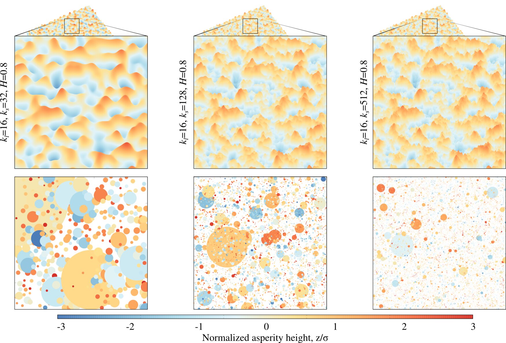
Fig. Identification of asperities on rough surfaces of different spectral content, the color of asperities corresponds to the vertical position of the summit and the size corresponds to the curvature radius; as could be easily seen from the figure, the higher the upper cutoff frequency is, the sharper the asperity summits are.
 Fig. 6 Contact between a spherical indenter and a deformable plane with a rough surface: we show the distribution of the contact area averaged over 2000 simulations for three values of the applied force, dashed lines represent the corresponding limits of the contact area predicted by the Hertz theory.
Version française (click to expand)
Contact entre un indenteur sphérique et un plan déformable à surface rugueuse : on montre la distribution de l’aire de contact moyennée sur 2000 simulations pour des trois valeurs de la force appliquée, la ligne pointillée représente la limite du contact prédit par la théorie de Hertz pour des surfaces lisses.
📚 References
- [23] V.A. Yastrebov. “The Elastic Contact of Rough Spheres Investigated Using a Deterministic Multi-Asperity Model”. Journal of Multiscale Modelling (2019), 10(1):1841002. [doi] [arXiv] [pdf]
🏠 Back to the Table of Contents
Elastic-plastic contact of rough surfaces
When numerical simulations possess several severe non-linearities, the difficulties associated with the numerical treatment of each of them are rather multiplied than simply summed up. It is especially true when the non-linear material behavior is not derived from a potential, but contains internal history variables. Therefore, numerical treatment of elasto-plastic contact of rough surfaces presents serious difficulties in terms of convergence. Therefore, in our in-house finite element suite Z-set we use a special algorithm to split non-linearities: the material non-linearity is not taken into account before the status of contact elements has not converged, which allows in most cases to increase the convergence robustness of the Newton method. The same method can be used with the Partial Dirichlet-Neumann (PDN) method, that I developed during my thesis, which relies on the active-set strategy the inequality contact constraints by equality ones and which operates exclusively on primal variables and nodal reaction forces [25]. These two improvements enabled us to solve complex normal-contact problems between a rigid flat and an elasto-plastic rough surface in large and small deformation formalisms.
From the theoretical point of view, the elasto-plastic contact of rough surfaces is much simpler than elastic one, since it is known that the contact pressure rapidly saturates at material hardness , which could be estimated to be , where is a certain yield-stress limit (either initial or saturated, depending on the hardening type). Therefore, the simplest elasto-plastic model for the true contact area evolution would be the model in which the area fraction is proportional to the nominal pressure :
This microscopic model is widely used in many macroscopic empirical laws where the contact area is required. However, this law is valid only for monotonic loading , which rarely happens in real engineering systems which rather operate under cyclic loading. But even if we assume a monotonic loading, a more accurate plastic law has to take into account the initial elastic deformation of asperities, which would result in an affine function of the area. Finally, under high pressures, which are relevant for machining, metal forming (rolling, drawing, stamping), and other demanding applications, the true contact area saturates at the nominal one, thus giving the following estimation for the contact area:
In our studies, with improved finite element algorithms, we could solve a series of elasto-plastic rough contact problems on real geometry [6], solve the viscous flow problem behind [26] and obtain a relatively good agreement with experimental results of Didier Lasseux (see Fig. 7). Moreover, we could construct a simple multi-asperity based model, which employs calibrated response of axisymmetric asperities and short range elastic interaction, to obtain quite accurate results, directly comparable with the heavy finite element simulations Fig. 8
In addition, in collaboration with Andreas Almqvist, Francesc Pérez-Ràfols and Andrei Shvarts we initiated a study aiming at comparing the boundary-element based method using an empirical algorithm to handle elasto-plasticity (the contact pressure is forced to remain in the interval ) [27] and the accurate finite element analysis. The main objective of this study was to demonstrate the ability of plastic deformations to erase small scale roughness, which would solve the fundamental problem in the elastic contact of rough surface – the necessity to introduce short wavelength cutoff. Regardless promissing results, this study has been remaining in idle state for few years already. Hopefully, it could be restarted soon. Globally, we have not obtained any groundbraking results but we demonstrated the capabilitiy of our computational tools to handle properly elasto-plastic contacts.
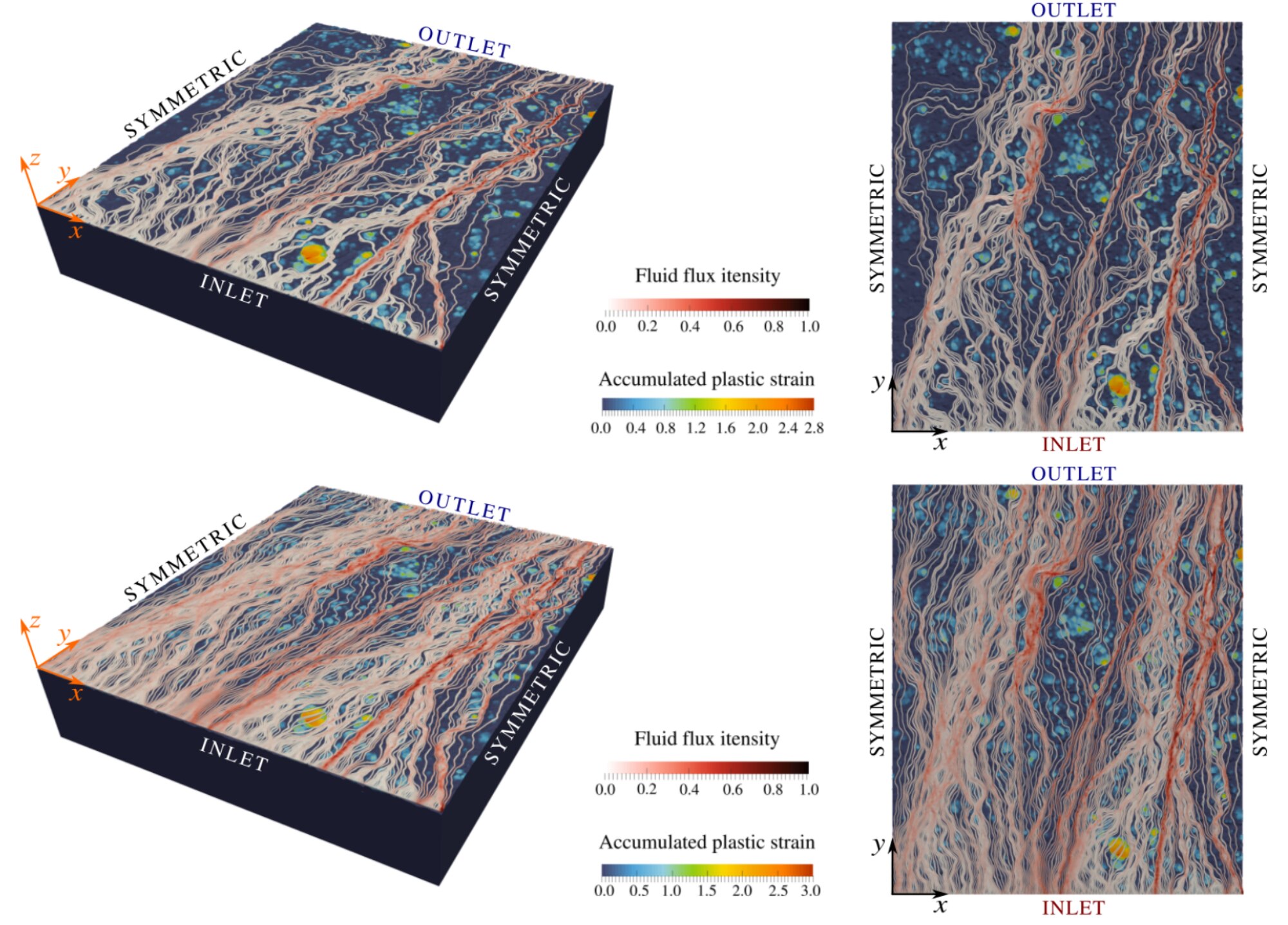
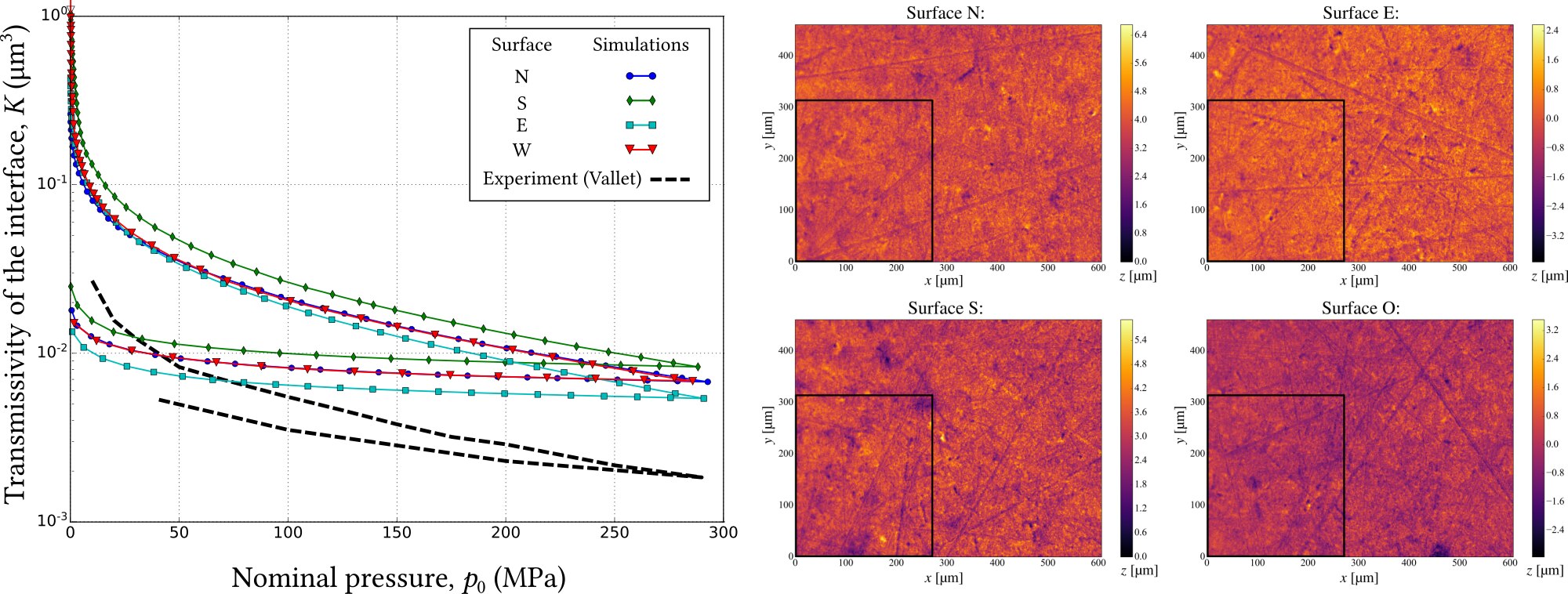 Fig. 7
Finite element simulation of elasto-plastic contact between a rough Stellite and a saphire plate [26]. Stream lines are coloured in red to highlight flux intensity, the blue-to-orange colour scale represents near surface accumulated plastic strain: the upper panel represents maximal loading, the middle panel shows the moment of separation (the plastic strain remains unchanged whereas the flux becomes more intense). In the lower panel shows comparison of four FE simulations with experimental results of Lasseux’s group [28].
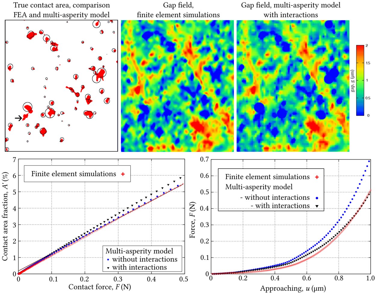 Fig. 8
Comparison of a full-scale finite element simulation results and a simplified multi-asperity model with and without elastic interactions between asperities, at the maximal load we compare: upper left - contact area, upper right - gap field, lower panel: area-force and force-displacement curves, results from [6] (at further stage of J. Durand’s thesis the detection algorithm for asperities was improved and the missing asperity identified by an arrow was incorporated in simulations).
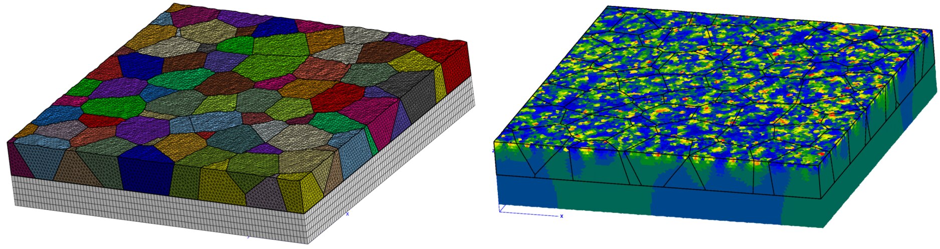
Finally, in the early stage of my career I worked a little bit on the contact of rough surface of polycrystalline aggregates, which rather validated the contact algorithms than permitted to obtain any physical insights into the topic. A simulation example is shown below: a finite element mesh with a polycristalline structure and the resulting cumulated plastic deformation after sever contact with a rigid flat.
📚 References
- [6] V.A. Yastrebov, J. Durand, H. Proudhon, G. Cailletaud. “Rough surface contact analysis by means of the Finite Element Method and of a new reduced model”. Comptes Rendus Mecanique, 339:473-490 (2011). [doi] [pdf]
- [26] A.G. Shvarts. “Coupling mechanical frictional contact with interfacial fluid flow at small and large scales” (2019). PhD thesis defended on March 20, 2019 at École des Mines de Paris in presence of the jury Res. Dir. D. Lasseux, Prof. M. Paggi, Prof. S. Stupkiewicz, Prof. J.A. Greenwood, Assist. Prof. V. Rey, Assist. Prof. N. Moulin, Prof. G. Cailletaud, Dr. J. Vignollet, Dr. V.A. Yastrebov. This PhD thesis was awarded by a 🏆 CSMA award for one of two best theses in computational mechanics and by 🏆 Hirn award for the best thesis in tribology.
[HAL] [pdf]
🏠 Back to the Table of Contents
Trapped fluid in contact interface
A classic study published in 1985 gives an impression that we fully understand how a sinusoidal surface of amplitude and wavelength behaves in the presence of a compressible lubricant under the action of normal pressure [29]. Among other things, it follows from this study that if the fluid is trapped, it has no possibility to escape the trap whatever the value of the pressure applied. In our study [30] with Andrei Shvarts we were able to demonstrate numerically and analytically (using the solutions of Flamant and Cerutti on the asymptotic expansion of the forces of fluid on a sinusoidal surface) that the Kuznetsov’s solution is not exact and that a fluid once trapped can escape by gradually opening the trap even in the context of small perturbations. The limit pressure for opening the trap within the limit of the infinitesimal slope converges to a very simple equation:
where is the volume of the fluid which, in the case of a compressible fluid, depends on the pressure, and where is the volume between two crests of the profile. For finite values of , the opening pressure is greater than this limit. Of course, for fluids with non-linear compressibility, up to two solutions can exist if the initial volume of the fluid is not less than the volume of the valley .
Even if the possibility for the fluid to escape the trap is interesting per se, this phenomenon is also important from practical point of view since it influences (1) the macroscopic friction, and (2) the behavior of engineering systems with trapped fluid under cyclic loading. The macroscopic coefficient of friction can vary in a strongly nonlinear and non-monotonic way depending on the constitutive behavior of the solid as well as of the fluid. The equation for the evolution of the macroscopic of friction could be obtained in a trivial way:
on the other hand, the expressions for the evolution of the fluid pressure and of the real contact area with respect to applied pressure are difficult to guess/deduce in the general case. We therefore used numerical simulations to explore different possible scenarios. We have shown that the macroscopic coefficient of friction can either decrease in a monotonic way or evolve in a more complex way (cf. Fig. 9(a) ). This discovery of the nonlinear relationship between the coefficient of friction and the pressure is a valuable result for tribology.
Another important consequence of the fluid entrapment is that in the presence of friction, high concentrations of shear stress can emerge under normal cyclic loading. This surprising result was revealed through numerical simulations, yet to explain it analytically we employed results from the linear elastic fracture mechanics (LEFM) for interface cracks at bi-material interfaces [31, 32] (cf. Fig. 9(b)). These high shear concentrations can cause an onset of fatigue cracks in vibration. Such cracks could be critical for vibrational resistance of some systems that must remain tightly sealed such as, for example, radioactive waste containers during transportation.
To construct our analogy between the LEFM and trap opening by the fluid, the following considerations were used. The fluid activation corresponds to the maximal extension of the contact zone (we shall denote the maximal contact half-length as , and during the subsequent increase of the external pressure the width of the contact zone is monotonically decreasing. For sufficiently small slope of the wavy profile, the situation corresponding to contact half-length can be considered as a configuration of two bonded dissimilar solids with two aligned semi-infinite interfacial cracks in the interface, separated by , see Fig. 9(b).
Using the superposition principle, the observed stress state, corresponding to the half-length of the contact patch , can be represented as a superposition of the initial shear traction , corresponding to the moment of activation of the fluid, and a stress induced by the same traction with the opposite sign, applied only on the surfaces of the cracks in the intervals , i.e. in the interval where the fluid penetrated. Such traction induces a singular shear stresses in the region between two cracks , thus can be written as:
where is the complex stress intensity factor, see [31, 32], and two terms in brackets in Eq. ??EQX??.2 correspond to two semi-infinite cracks being considered, so that , is the imaginary part. Therefore, the resulting distribution of shear tractions is given by the superposition . The complex stress intensity factor is calculated using the existing analytical formula for considered configuration and shear traction distribution [31, 32]:
where
and the parameter accounts for the different properties of the two bonded solids, in case one of them being rigid, it equals to
A sound similarity is found between numerical results and analytical formulae provided by the LEFM.
Therefore, we have shown that during the process of trap opening due to increasing pressure in the fluid with friction taken into account, the tangential tractions near the contact edges are elevated up to the limit provided by the Coulomb friction law. Consequently, even if the majority of the interface remains in stick state, local slip zones emerge at the boundaries of contact zones. It is important to account for such an elevated shear stress near edges of contact zones, which surround trapped fluid, in the analysis of damage evolution and crack onset under monotonic and cycling loading, including fretting fatigue [33, 34].
Version française (click to expand)
Une étude classique publiée en 1985 donne l’impression que l’on comprend bien comment se comporte une surface sinusoïdale d’amplitude et longueur d’onde en présence d’un lubrifiant compressible sous l’action d’une pression normale [29]. Entre autres, il suit de cette étude que si le fluide est piégé, il n’a pas de possibilité de s’échapper quelle que soit la valeur de la pression appliquée. Dans notre étude [30] avec Andrei Shvarts nous avons pu démontrer numériquement et analytiquement (en utilisant les solutions de Flamant et Cerutti sur l’expansion asymptotique des efforts de fluide sur une surface sinusoïdale) que la solution de Kuznetsov n’est pas exacte et qu’un fluide une fois piégé peut s’échapper en ouvrant graduellement le piége même dans le contexte de petites perturbations. La pression limite d’ouverture du piège dans la limite de la pente infinitésimale converge vers une forme très simple :
où est le volume de fluide qui, dans le cas d’un fluide compressible, dépend de la pression, et où est le volume compris entre deux crêtes de la sinusoïde. Pour des valeurs finies de , la pression d’ouverture est supérieure à cette limite. Bien entendu, pour des fluides à compressibilité non-linéaire, jusqu’à deux solutions peuvent exister si le volume initial de fluide n’est pas inférieur au volume de la vallée .
La possibilité d’échappement du fluide est intéressante en soi, mais de plus ce phénomène influence (1) le frottement macroscopique, et (2) le comportement des systèmes comportant des fluides piégés sous un chargement cyclique. Le coefficient de frottement macroscopique peut varier d’une manière très non linéaire en fonction du comportement du solide ainsi que du fluide. L’équation de ce changement est obtenue de façon triviale :
par contre, les expressions de la pression de fluide et de l’aire de contact réelle en fonction de la pression appliquée sont difficiles à déduire dans le cas général. Nous avons donc recouru à des simulations numériques pour explorer les différents scénarios possibles. Nous avons montré que le frottement macroscopique peut décroître d’une manière monotone ou bien évoluer d’une manière plus complexe (cf. Fig. 9(a)). Cette découverte de la relation non linéaire entre le coefficient de frottement et la pression est un résultat intéressant pour le monde de la tribologie.
Une autre conséquence importante du piégeage des fluides est qu’en présence de frottement, de fortes concentrations de contrainte de cisaillement peuvent émerger sous chargement normal cyclique. Cette conclusion insolite a été obtenue numériquement mais nous l’avons également expliquée analytiquement en faisant le recours à la mécanique linéaire de la rupture le long des interfaces bi-matériaux [31, 32] (cf. Fig. 9(b)).
Ces fortes concentrations de cisaillement peuvent provoquer l’amorçage de fissures de fatigue en vibration, qui peuvent être critiques pour certains systèmes qui devrait rester fortement étanches comme, par exemple, des conteneurs de déchets radioactifs lors du transport.
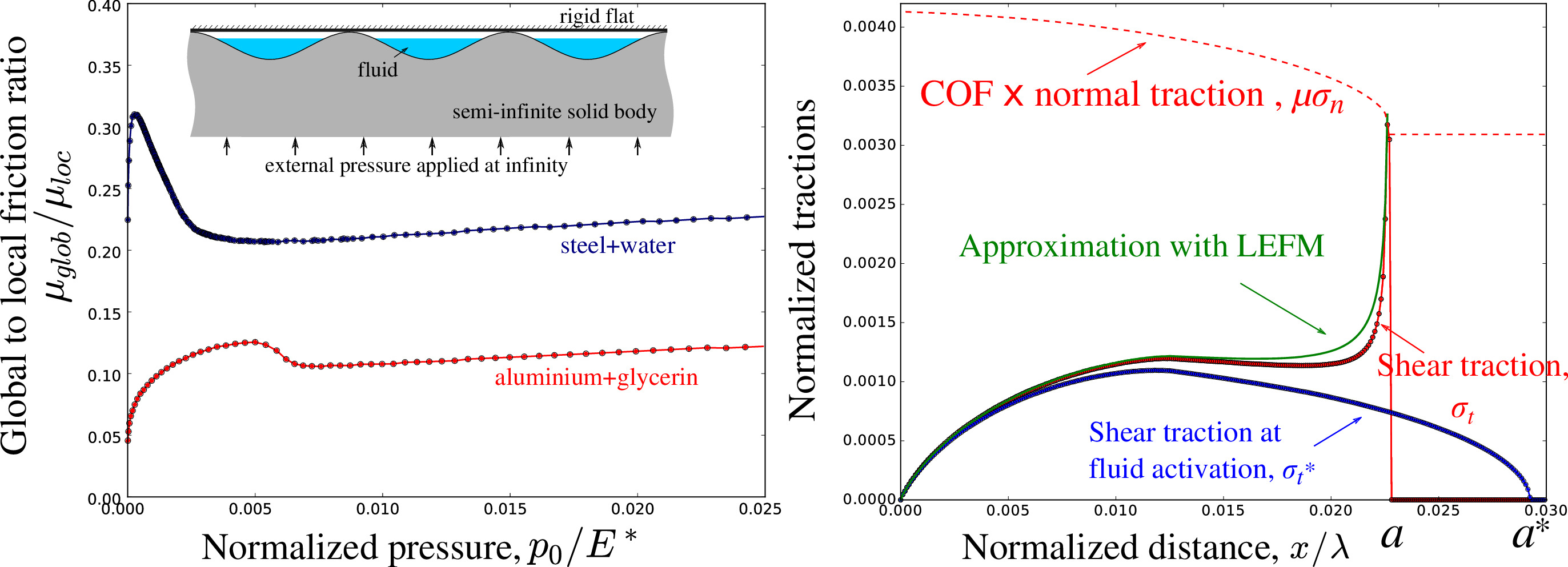 Fig. 9
(a) Evolution of the friction coefficient for (i) steel/water and (ii) aluminum/glycerol combinations; (b) illustration of the high concentration of shear stress that arises near the contact edge upon increase in normal pressure accompanied by fluid expansion in the contact interface; comparison with the analytical solution inspired by the linear elastic fracture mechanics.
Version française (click to expand)
(a) Évolution du coefficient de frottement pour des combinaisons (i) acier/eau et (ii) aluminium/glycérol ; (b) illustration de la forte concentration de la contrainte de cisaillement qui surgit près du bord du contact lors de l’augmentation de la pression normale accompagnée par l’expansion du fluide dans l’interface de contact ; comparaison avec une solution analytique provenant de la mécanique linéaire de la rupture.
📚 References
- [30] A.G. Shvarts, V.A. Yastrebov. “Trapped fluid in contact interface”. Journal of the Mechanics and Physics of Solids, 119:140-162 (2018). [doi] [arXiv] [pdf]
🏠 Back to the Table of Contents
Creeping fluid flow in contact interface between rough surfaces
Representativity of rough surfaces in mechanical contact is of great importance, yet it is even more relevant for studies of permeability of contact interfaces especially for low and high pressures. This representativity becomes crucial to numerically studies near the percolation point associated with the existence of an infinite contact cluster. On the other hand, the finite element method is a CPU-time demanding tool for studies of rough surfaces with a sufficiently rich spectrum. Moreover, in many application problems, the strong coupling between the equations of the mechanics of solids and fluids is not necessary because the pressure in the fluid is lower by several orders of magnitude than those which develop in the contact. In this case, a framework much less greedy in terms of time and computing power can be used: this is the boundary element method. By adopting the one-sided coupling between the boundary element method responsible for the mechanical contact and the finite element method used to solve the Reynolds equation on the topography found by the first, we were able to tackle this interesting problem which is relevant for numerous applications, notably for systems where the tightness is ensured by the static contact (cf. Fig. 10).
Show animation.
Under increasing pressure, the non-conducting area including contact zones and trapped fluid, shown in navy color, grows smoothly in the beginning and in a step-wise manner closer to the percolation. Main flow channels shown in red change their morphology and intensity (the flux intensity at every frame is normalized by the maximal value).
By covering a wide range of roughness parameters, through thousands of simulations to capture the stochastic nature of the topography, we were able to establish a phenomenological law between the normalized interface permeability and the normal pressure , which allows us to define the average flux as a function of the hydrostatic pressure drop over a distance :
where is the dynamic viscosity of the fluid, is the -th spectral moment and is the effective modulus of the contact between two elastic solids. The two constants and are determined by numerical simulations and remain fairly invariant for all the surfaces studied.
This phenomenological law is applicable within the exponential-decay regime for not too low pressures but well below the permeability pressure.
Besides this law, other important results have been obtained. For example, we showed that the self-consistent homogenization model applicable to the study of the permeability of contact interfaces, and which is based on the probability distribution of film thickness (equal to the aperture value), should include a correction to ignore the pockets of trapped fluid [35]. The normalized permeability , it could be found from the corrected equation:
where is the gap, its probability density and is the non-conductive contact area including the contact area and trapped fluid. The probability density of the gap field was studied in [36], but we could obtain much more clean and statistically meaningful distributions and suggest their functional shape, which could help in analytical estimation of permeability [37].
In addition, we have analytically estimated [37] the asymptotic distribution of the film thickness in the vicinity of zero “gap” for a parabolic indentor of radius of curvature and for a contact patch of radius :
The factor of this distribution will of course be modified for a contact area composed of several contact "spots".
In the geometric intersection model (Winkler foundation), the linear size of the contact clusters scales as , where is the Hurst exponent [38, 14], this "scaling" remains approximately valid for accurate contact models including elastic interactions: at least for , it was found that [39]. By integrating over all contact points (the smallest linear cluster size was added) will provide a factor to the probability distribution of the "gap" but will not modify the power law which has been recently demonstrated in another way in [40].
Finally, using a more elaborated – strongly coupled – fluid-solid computational framework, based on numerous simulations, we deduced a novel non-local permeability law [26], Sec. 9.3, pp. 155-158:
where is the normalized permeability, is the external pressure, is the average fluid pressure and is its gradient, is the effective elastic modulus, and are dimensionless parameters and is the characteristic length scale. Naturally should be very close to unity, whereas the characteristic length depends on the roughness parameters. This non-local permeability law implies that the fluid flux depends not only on the local difference in applied and fluid pressures but also on the gradient of the latter.
Version française (click to expand)
La représentativité des surfaces rugueuses dans les études du contact mécanique est très importante, mais elle est encore plus pertinente pour des études de perméabilité des interfaces de contact surtout pour de faible et de forte pressions. Cette représentativité devient cruciale pour étudier numériquement des phénomènes près du point où se produit la percolation associée avec l’existence d’un cluster infini de contact. Par contre, la méthode des éléments finis est un outil très coûteux pour des études des surfaces rugueuses à spectre suffisamment riche. De plus, dans beaucoup de problèmes applicatifs, le couplage fort entre les équations de la mécanique des solides et des fluides n’est pas nécessaire car la pression dans le fluide est inférieure de plusieurs ordres de grandeur de celle qui se développe dans les zones de contact. Dans ce cas, un cadre beaucoup moins gourmand en termes de temps et de puissance calcul peut être utilisé : c’est la méthode des éléments de frontière. En adoptant, le couplage unilatéral entre la méthode des éléments de frontière responsable pour le contact mécanique et la méthode des éléments finis utilisée pour résoudre l’équation de Reynolds sur la topographie trouvée par la première, nous avons pu aborder ce problème intéressant et fort important pour des systèmes où l’étanchéité est assurée par le contact statique entre des surfaces (cf. Fig. 10).
En couvrant une large plage de paramètres de rugosité, grâce à des milliers de simulations afin de capturer la nature stochastique de la topographie, nous avons pu établir une loi phénoménologique entre la perméabilité normalisée de l’interface et la pression normale , qui permet de définir le flux moyen en fonction de la chute de la pression hydrostatique sur une distance :
où est la viscosité dynamique du fluide, est le -ième moment spectral et est le module effectif du contact entre deux solides élastiques. Les deux constantes et sont déterminées par des calculs numériques et restent assez invariables pour toutes les surfaces étudiées.
Cette loi phénoménologique est applicable dans le régime de décroissance exponentielle pour des pressions pas trop faibles mais bien inférieures à la pression de perméabilité.
A part de cette loi, d’autres résultats importants ont été obtenus. Par exemple, nous avons démontré que le modèle auto-cohérent d’homogénéisation applicable à l’étude de la perméabilité des interfaces de contact, et qui se basent sur la distribution de probabilité d’épaisseur du film (égale à la valeur d’ouverture), devrait comporter une correction pour ignorer les poches de fluide piégé [35]. De plus, nous avons estimé [37] analytiquement la distribution asymptotique d’épaisseur du film au voisinage de zéro “gap” pour un indenteur parabolique du rayon de courbure et pour une tache de contact de rayon :
Le facteur de cette distribution sera bien entendu modifié pour une aire de contact composée de plusieurs "spots" de contact.
Dans le modèle d’intersection géométrique (fondation de Winkler), la taille linéaire des clusters de contact se dimensionne comme , où est l’exposant de Hurst [38, 14], ce "scaling" reste approximativement valable pour des modèles de contact précis incluant des interactions élastiques : au moins pour , il a été trouvé que [39]. En intégrant sur tous les points de contact (la plus petite taille linéaire de cluster était ajouté) fournira un facteur à la distribution de probabilité du "gap" mais ne modifiera pas la loi de puissance qui a été recemment démontré d’une autre façon dans [40].
Même si des surfaces à spectre riche sont pas accessibles à la méthode des éléments finis, nous avons fait une étude numérique de perméabilité des interfaces de contact entre surfaces rugueuses dans notre cadre monolithique développé pour ces problèmes fortement couplés. Nous avons établi une autre loi phénoménologique de perméabilité non locale. La non-localité dans ce cas se traduit par la dépendance de la perméabilité, pas seulement en fonction de la pression et de la pression de fluide mais encore en fonction du gradient de pression de fluide . Cette loi a été identifiée pour la composante du tenseur de perméabilité colinéaire avec la direction de , sous la forme suivante :
où sont des nombres adimensionnels (universels dans la plage étudiée des paramètres) qui ont été déduits des simulations numériques et est la longueur caractéristique.
Le travail sur cette loi n’est pas encore terminé, mais potentiellement il pourrait améliorer la précision des études de perméabilité des systèmes de fissures complexes saturées en compression qui font l’objet d’études en hydrogéologie.
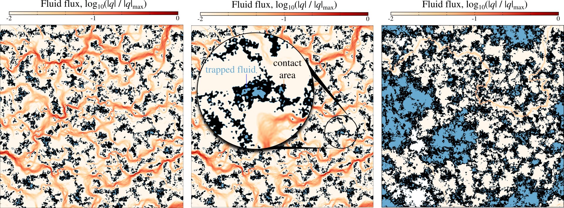 Fig. 10 Viscous fluid flow through the contact interface shown in reddish color scale, contact area shown in black and trapped fluid shown in blue. Two configurations are shown for relatively small contact area and much larger contact area showing large portions of fluid trapped.
Version française (click to expand)
Flux d'écoulement dans l'interface de contact. Les taches de contact sont noires, le fluide piégé est en bleu. Deux instances sont présentées qui correspondent à des différentes valeurs de pression.
📚 References
- [35] V.A. Yastrebov, G. Anciaux, J.F. Molinari. “Permeability of the contact interface between rough surfaces” (2021) in the final stage of writing, draft is provided [encrypted pdf]
- [37] V.A. Yastrebov, G. Anciaux, J.F. Molinari. “Gap distribution in contact interfaces between rough surfaces and transmissivity analysis” (2021) in the final stage of writing, draft is provided [encrypted pdf]
- [26] A.G. Shvarts. “Coupling mechanical frictional contact with interfacial fluid flow at small and large scales” (2019). PhD thesis defended on March 20, 2019 at École des Mines de Paris in presence of the jury Res. Dir. D. Lasseux, Prof. M. Paggi, Prof. S. Stupkiewicz, Prof. J.A. Greenwood, Assist. Prof. V. Rey, Assist. Prof. N. Moulin, Prof. G. Cailletaud, Dr. J. Vignollet, Dr. V.A. Yastrebov. This PhD thesis was awarded by a 🏆 CSMA award for one of two best theses in computational mechanics and by 🏆 Hirn award for the best thesis in tribology.
[HAL] [pdf]
🏠 Back to the Table of Contents
Coupled flow through a wavy channel
With some fairly strong assumptions, we were able to propose an analytical solution that describes the coupled flow of a viscous fluid along an elastic body with a sinusoidal surface brought into contact with a rigid plane [41]. This solution takes into account the deformation of the substrate by the contact forces and by the fluid pressure; the associated Reynolds equation is solved on the updated geometry. The solution predicts the average pressure in the fluid along the channel of length subject to the external pressure , and the inlet and outlet fluid pressures :
with being the amplitude and being the wave-length, and the function is given by
Using this solution, we can derive the flux at each point, which gives the equation
which in turn, after integrating provides us with the mean flow, which is in very good agreement with the results of the strongly coupled finite element calculation (see Fig. 11).
We believe that this solution for a three-dimensional coupled fluid/solid/contact problem represents a rare example of an approximate analytical solution for such complex problems.
The associated numerical solution allows us to go well beyond the validity range of the analytical solution, and allowed us to predict the critical channel closure pressure, which depends only on the geometry , the elastic parameters and, surprisingly, only on the inlet fluid pressure and not on the outlet one. The resulting closing pressure is given by:
Version française (click to expand)
Avec quelques hypothèses assez fortes, nous avons pu proposer une solution analytique qui décrit l’écoulement d’un fluide visqueux le long d’un corps élastique à surface sinusoïdale mis en contact avec un plan rigide [41]. Cette solution prend en compte la déformation du substrat par les efforts de contact et par la pression dans le fluide ; l’équation de Reynolds associée est résolue sur la géométrie actualisée. La solution prédit la pression moyenne dans le fluide le long du canal de longueur soumis à la pression externe , et des pressions du fluide d’entrée et de sortie :
étant l’amplitude d’ondulation et étant la longeur d’onde, avec
En utilisant cette solution, nous pourrons dériver le flux en chaque point, ce qui donne l’équation
qui après une intégration fournit le flux moyen, qui se compare très bien avec les résultats du calcul par élément finis fortement couplé (cf. Fig. 11).
Cette solution pour un problème couplé fluide/solide/contact à trois dimensions représente un rare exemple de solution analytique approchée pour des problèmes aussi complexes.
La solution numérique associée permet d’aller bien au-delà du domaine de validité de la solution analytique, ce qui nous a permis de prévoir la pression critique de fermeture du canal, qui ne dépend que de la géométrie , des paramètres élastiques et de la pression de fluide d’entrée :
 Fig. 11 Effective transmissivity of a channel formed by a sinusoidal surface in contact with a rigid plane. Within its validity range, our analytical solution compares well with the results of the strongly coupled solid/fluid finite element calculation.
Version française (click to expand)
Transmissivité effective d’un canal formé par une surface sinusoïdale mise en contact avec un plan rigide. Dans son intervalle de validité, notre solution analytique se compare bien avec les résultats du calcul éléments finis solide/fluide fortement couplé.
📚 References
- [41] A.G. Shvarts, V.A. Yastrebov. “Fluid flow across a wavy channel brought in contact”. Tribology International, 126:116-126 (2018). [doi] [arXiv] [pdf]
🏠 Back to the Table of Contents
Electric contact between rough surfaces
 Experimental set-up for the study of roughness-induced contact electric resistance.
In the framework of postdoc of Frederick Sorel Mballa Mballa co-supervised by Georges Cailletaud, Henry Proudhon, Frédéric Houzé and Sophie Noël funded by Labex LaSIPS we worked on the electric contact in ball/substrate configuration taking into account surface roughness as well as accurate material models. Nonlinear material models for brass substrate as well as for nickel and gold micron-thickness electroplated coatings were properly calibrated, beryllium bronze of the ball indenter was assumed to be elastic. plasticity was used for all substrate materials with a single kinematic hardening for nickel and gold whereas for the brass it was supplemented with two other kinematic hardening rules as well as with the isotropic hardening. However, even such an elaborated model of the brass was not enough to capture the experimentally measured resistance/force hysteresis loops [42], we demonstrated that the thickness of Ni and Au layers was not crucial for this analysis. Nevertheless, in this project we successfully combined three different models to estimate the electric resistance of contact interfaces Fig. 12:
-
macroscopic (smooth surfaces) finite element simulation of indentation with advanced material modelling which provided us with the macroscopic force/displacement/area curves;
-
experimental roughness analysis which was taken into account at the microscopic scale to model the distribution of conductive spots, we used an iterative elasto-plastic model of interacting contact spots which in mean-field sense has to verify the the macroscopic pressure and contact area obtained in model 1.;
-
to estimate the evolution of the electric contact resistance of the resulting contact interface, we used Greenwood’s model [43]:
where is the effective resistivity, is the size of -th contact spot and is the distance between -th and -th spots.
In addition, a full scale 3D finite element model incorporating surface roughness and all material models was constructed and solved for relevant loading conditions, however, the final thermal analysis was not conducted Fig. 12, therefore these results remain unpublished. Hopefully, this work could be finalized in the framework of PhD thesis of Paul Beguin on the thermal contact.
Regardless all our efforts to match the experimental resistance via modelling, our results were located on the minimal level of resistance identified in experiments and only upon using the hardest version for the brass’ yield stress ( MPa). The most convincing hypothesis of this discrepancy is the presence of non-conductive oxidized zones on the side of beryllium bronze ball, which has to considerably increase the electric resistance. In perspective, it would be interesting to restart this project keeping the same materials of the substrate but ensuring a coating of the bronze balls with a gold layer to ensure conductivity of all contact spots.
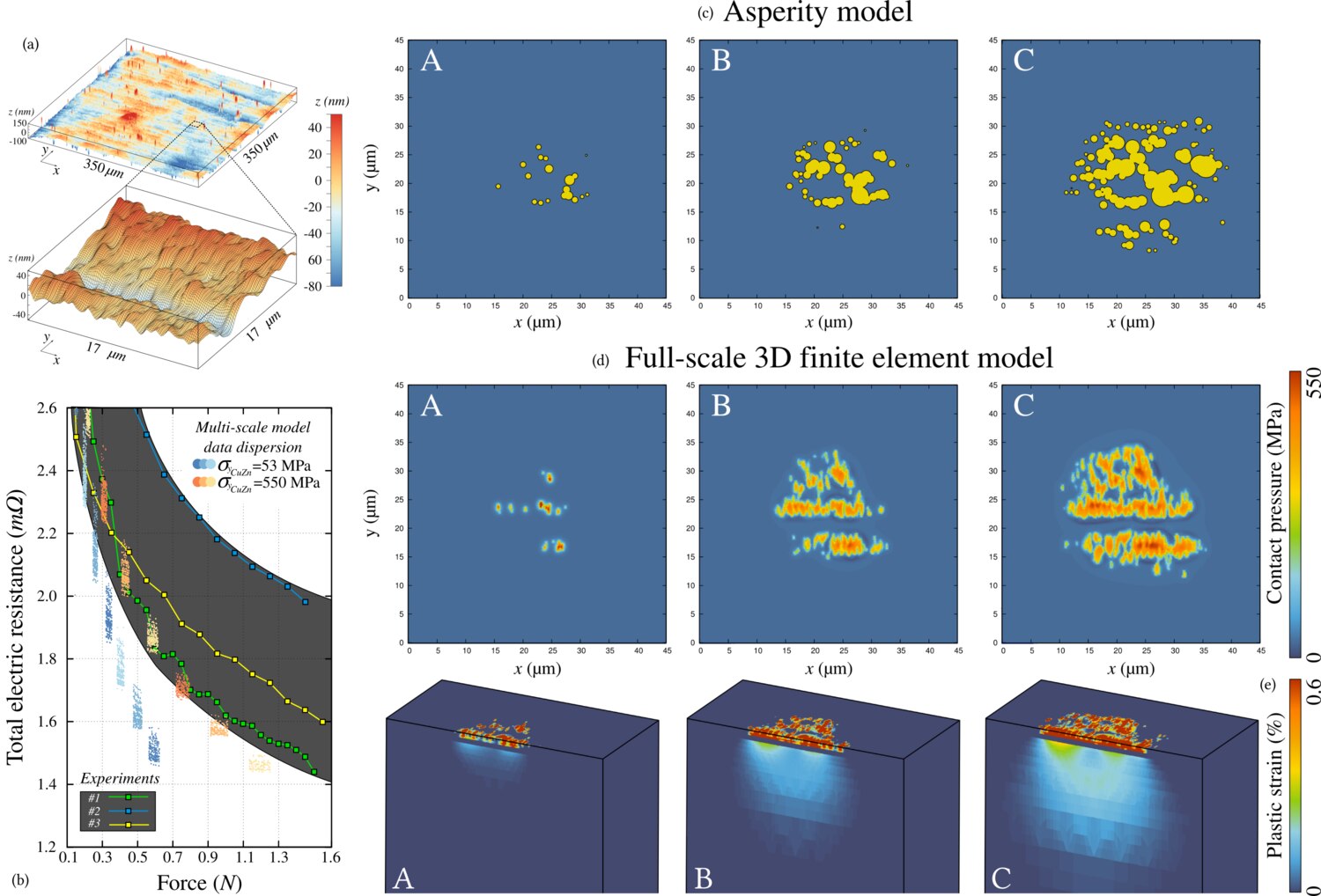 Fig. 12
(a) a characteristic surface roughness of rolled brass after being electroplated with nickel and gold (AFM) which was used in (c ) multi-scale model employing multi-asperity elasto-plastic contact model and (d-e) direct finite element analysis of mechanical contact, in (e) a cut through the substrate is shown to highlight plastic deformations of the brass; (b) contact resistance results of the three-level (multi-scale) model (clouds of points obtained in numerous simulations of rough surface locations) compared to experimental results (dashed area and three particular curves). Note that figures (c ) and (d) cannot be compared directly because they do not correspond to exactly the same location on the rough surface. As seen in (e) nickel layer (thin line separating two plastically deformed media: gold coating and brass substrate) remains in elastic regime.
📚 References
- [42] V.A. Yastrebov, G. Cailletaud, H. Proudhon, F.S. Mballa Mballa, S. Noël, Ph. Testé, F. Houzé. “Three-level multi-scale modeling of electrical contacts: sensitivity study and experimental validation”. In Proceedings of the Holm 2015 61st IEEE Holm Conference on Electrical Contacts, pp. 414-422 (2015). [doi] [pdf]
- Presentation “Three-level multi-scale modeling of electrical contacts” constructed together with Georges Cailletaud and given by him at the 61st IEEE Holm Conference on Electrical Contacts, San Francisco, USA. 14 October, 2015 [pdf]
🏠 Back to the Table of Contents
Greenwood’s elliptic model
In simplified elliptic model of rough contact recently suggested by James A. Greenwood [24] the asymptotic solutions obtained by the author are valid only for small values on Nayak’s parameter , which is not representative for real rough surfaces. We derived a better asymptotic solution valid for higher values of this parameter.
According to Greenwood’s simplified elliptic model of rough surface contact, the true contact area fraction and the mean pressure are given by the following equations, respectively
where , is the normalized separation between the effective rough surface and a rigid flat, is the normalized geometric mean curvature, is the variance of roughness, is the variance of the roughness gradient, is the effective elastic modulus, and is the Nayak’s parameter with being the fourth spectral moment of the isotropic normal roughness. The joint probability of asperities with the summit at normalized elevation and the normalized mean geometric curvature was obtained by Greenwood as
So it was shown by Greenwood that for large separations , the asymptotic solutions for pressure and area are given by
After some algebra, we showed that the true asymptotics for high values of Nayak parameter are given by the following expressions:
 Fig. 13
True contact area evolution with Nayak’s parameter as predicted by simplified elliptic model [24]: (a) classical normalization Eq. [10, 24] valid only for small and huge separations , (b) new normalization Eq. valid for big and arbitrary separation .
 Fig. 14
Nominal pressure evolution with Nayak’s parameter as predicted by simplified elliptic model [24]: (a) classical normalization Eq. [10, 24] valid only for small and huge separations , in the inset zoom on the region of moderate where the minimum value of the nominal pressure is reached; (b) new normalization Eq. valid for big and reasonable separations .
📚 References
- Yastrebov, V.A. “Some observations on Greenwood’s simplified elliptic model of rough contact”, this short note is in a draft stage.
🏠 Back to the Table of Contents
Size and material effects in indentation
The power law decay of the roughness power spectral density (PSD) is approximately preserved down to the sub-micron scale [44], where various size effects in material deformation become pronounced.

Fig. Various size effects justifying the difference between near surface small-scale contact and macroscopic or structural-scale contact: thin coatings, oxide layer, grain size due to work-hardening, surface energy.
Therefore with Samuel Forest, and now in interaction with Vikram Phalke we studied size effects in normal deformation of small asperities. It is known that, contrary to sharp indenters which demonstrate different hardness for different penetration depths [45, 46], smooth indenters demonstrate the size effect with the radius of their curvature [47]:
where is the material hardness for the indenter of radius , is the macroscopic hardness and is the characteristic curvature radius (material parameter). This size effect if not easy to capture in computational models, and our first attempt undertaken, in which we used Cosserat continuum in axisymmetric configuration, was unsuccessful. Rather expectedly, while varying elastic and plastic characteristic lengths [48] we could capture a saturated small-scale response, large-scale response and a smooth transition between them, but we could not show an increasing hardness for decreasing size of the indenter: the hardness remained almost constant for all and . More specifically, both the nominal pressure and the relative contact radius were shown to increase for a given indentation under decreasing indenter radius , however, their ratio remains unchanged see Fig. 15.
 Fig. 15
Nevertheless, we could demonstrate a characteristic change in accumulation of plastic deformation: for smaller curvature radii the plastic deformation accumulates near the surface whereas for larger radii, the plastic accumulation follows a classical under-surface onset and plastic core growth (see animations below). Currently we are working with more advanced gradient plasticity models with the objective to capture size effects in isotropic and homogeneous () and in crystal plasticity. Another study on the indentation of a single crystal where experimental results were compared with finite element simulations could be mentioned here [49], however, my participation in this study was very marginal: I simply assisted Prajwal Sabnis in contact simulations of this indentation.
Show animation.
 Accumulated plastic strain for two different indentation radii $R=2$ $\mu$m and $R=20$ $\mu$m.
A simple empirical size-dependent model was created at the asperity scale and thanks to my multi-asperity framework with elastic interactions, I could solve indentation of rough surfaces by a spherical indenter (see Fig. below). However, the lack of macroscopic plastic deformation in this study render it slightly artificial, so these results were not published.
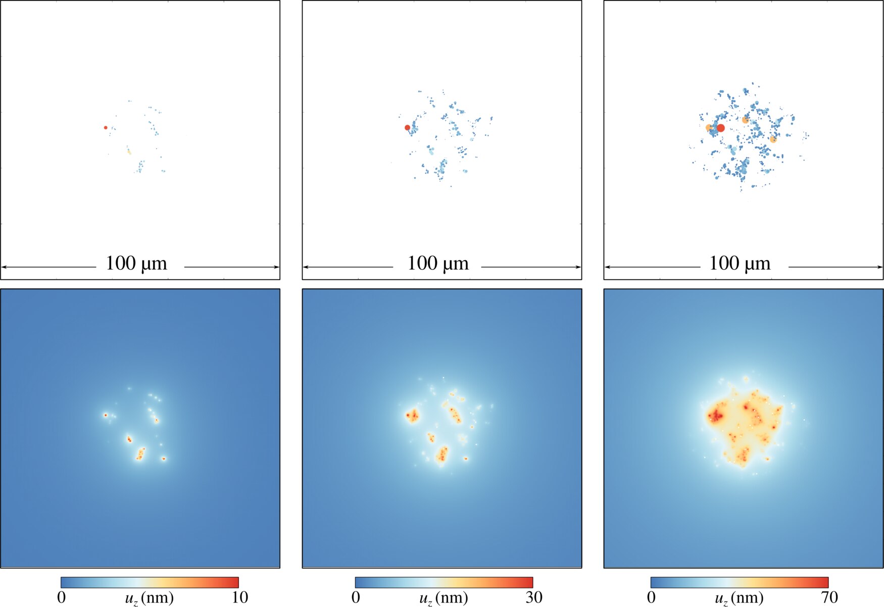
Fig. Deformation of a rough surface under spherical indentation taking into account size-dependent elasto-plastic deformation of elastically-interacting asperities: upper panel - view of contacting asperities, lower panel - total deformation of the substrate.
📚 References
- [49] P. A. Sabnis, S. Forest, N. K. Arakere, V.A. Yastrebov. “Crystal plasticity analysis of cylindrical indentation on a Ni-base single crystal superalloy”. International Journal of Plasticity, 51:200-217 (2013). Note: my participation to this study was very marginal. [doi] [pdf]
- V.A. Yastrebov, S. Forest “Mechanical contact between rough elastic-plastic solids: scale effect in deformation of asperities” In book of abstracts 52th SES technical meeting Texas A&M, College Station, USA, 25-29 October (2015). [pdf]
🏠 Back to the Table of Contents
Model for electric-arc-induced damage in contactors
In the thesis of Aurélien Fouque we studied degradation of AgSnO contactors under repetitive action of electric arcs. An intense experimental campaign carried out by Aurélien and Schneider Electric allowed us to measure to which extend the demixing is related to the arc power and duration, what is the shape of the crater, what is the maximal depth of melting pull, which is characterized by different recrystallized microstructure [50], what is the chemical composition of the near surface layer after the impact, etc. Long multi-arc experiments (up to 50,000 arcs) enabled us to follow the evolution of the demixed layer, which goes far beyond the maximal melting depth. Therefore, we deduced that the growth of the demixed silver layer must be accompanied with the silver transfer from one electrode to another. All these data was incorporated in a model which can handle:
- elasto-plastic contact with and without elastic interactions on realistic geometries,
- demixing of AgSnO,
- hardness dependence on the SnO content,
- increased porosity of solidified AgSnO and increased material loss due to projection of droplet of demixed Ag,
- topographical changes due to crater formation at a random point within the contact area of the previous contact,
- silver transfer from one contactor to another by debonding,
- final welding corresponding to a large enough contact area (the energy of the opener is below the one needed to break the weld).
The resulting model calibrated on experimental data could reproduce many aspects related to the deterioration of contactors leading to the ultimate welding. In this study, I followed the experimental campaign from a distance, but I took the lead in the development of the multiphysical model. In Fig. 16 and the animation below one could see how the contact area, surface topography, as well as demixing on both electrodes, every 50th cycle is shown. In Fig. 17, one could see the cut through the multi-arc model showing the amount of demixed silver compared with SEM images after the same number of cycles, the maximal depth measured in simulations and experiments is also shown.
Show animation.
Animation demonstrating how according to our multi-arcs demixing model evolve the microtructure (AgSnO composite transforms into pure Ag, while particles of SnO are either ejected with droplets or segregated in compact layers) and the surface topography.
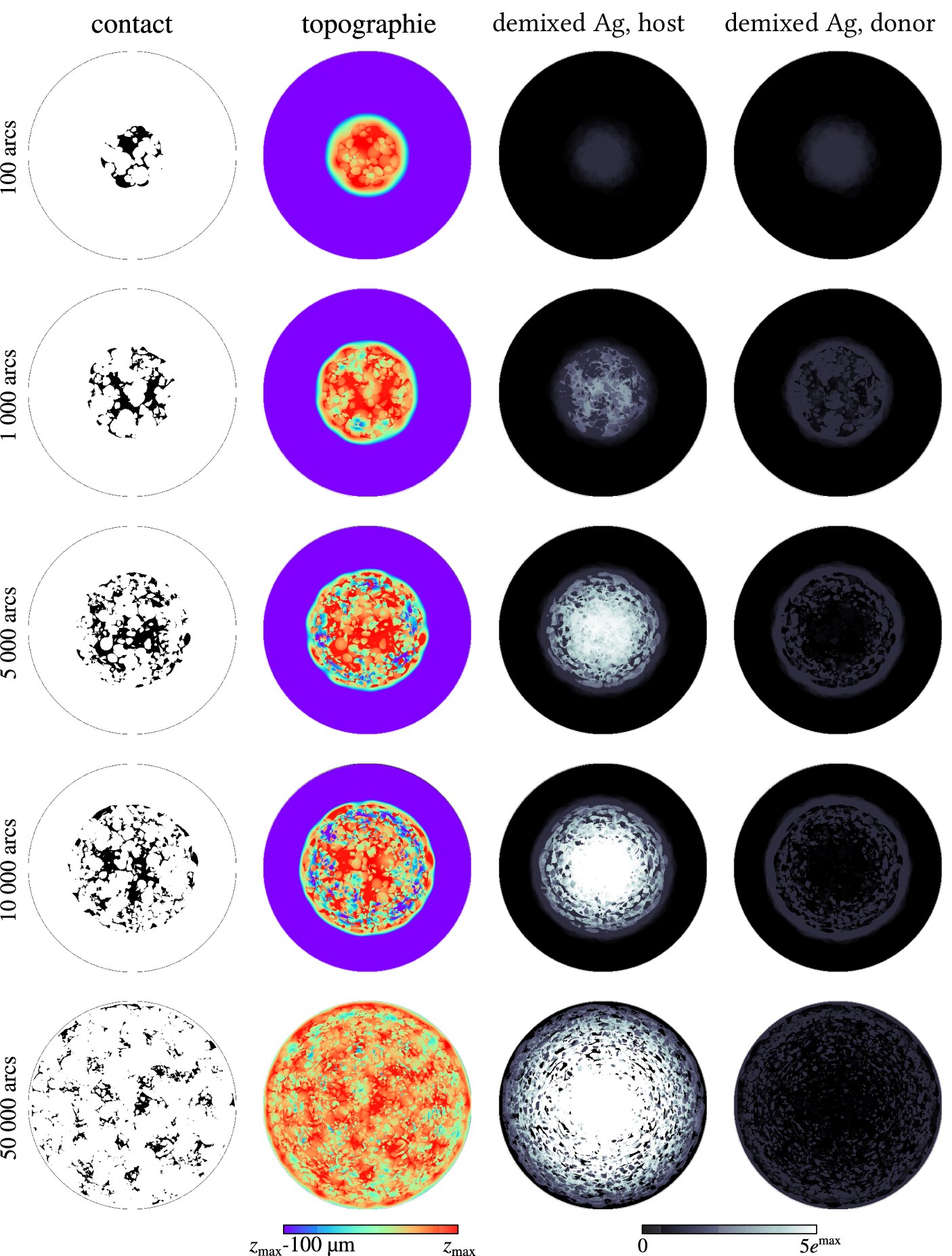 Fig. 16 Results of the multi-arc demixing model, from left to right: contact area, effective surface topography, demixed silver on the host-electrode and on the donor-electrode.
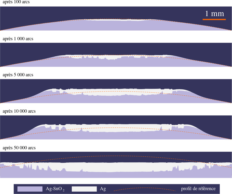
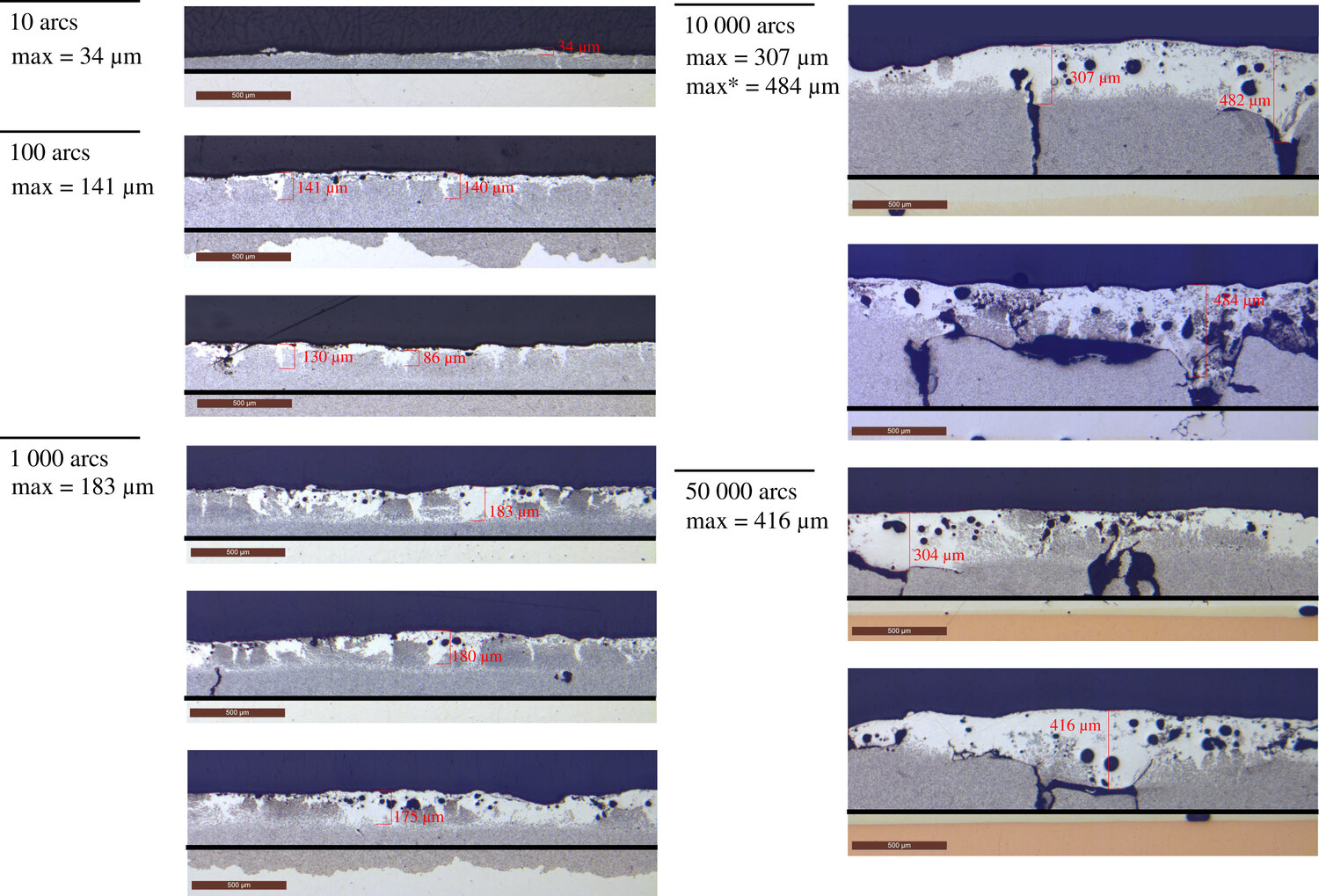
Fig. 17 On the left – cut through a model showing the topography and the amount of demixed silver after different number of arc’s impacts, on the right – experimental images (SEM) showing the demixing of the silver in one of electrodes after different number of arc’s impacts.

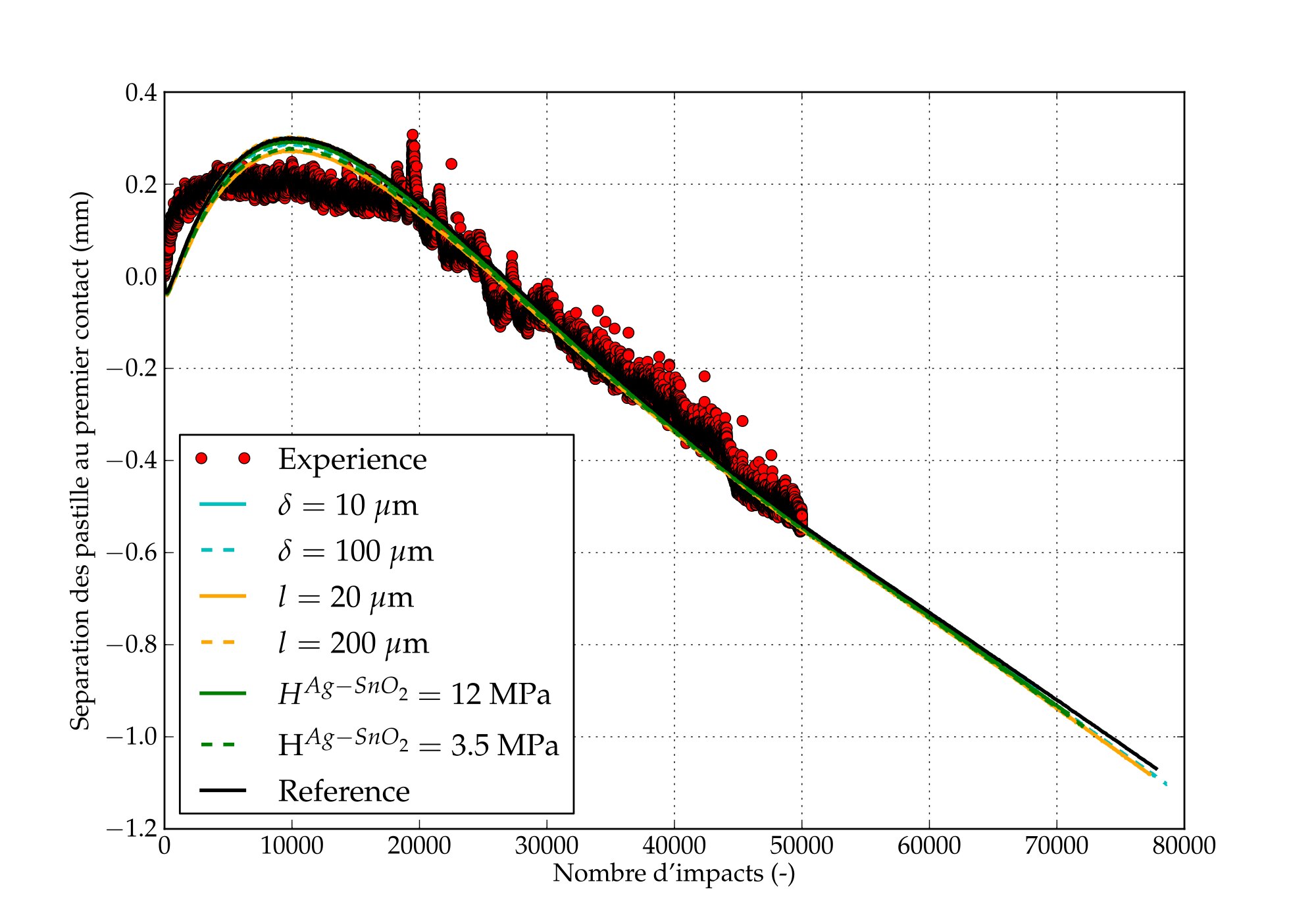
Fig. A parametric study demonstrating how the maximal silver penetration depth evolves with the number of arcs: (left) – experimental data and model prediction for different parameters are shown, (right) – evolution of the distance between two closed electrodes under the same squeezing force demonstrates the initial material swelling (due to induced porosity) and further material loss (due to the decrease of viscosity in the pure silver liquid phase).
📚 References
- A. Fouque. Contribution à l’étude du couplage thermique-mécanique-électrique dans les contacts électriques : application à l’élaboration d’un modèle de durée de vie d’un contacteur. PhD thesis, Paris-Saclay University (2020). PhD advisors: G. Cailletaud, V. Esin (MINES ParisTech) & F. Houzé, Ph. Testé, R. Landfried (GeePS, CentraleSupélec) in collaboration with Schneider Electric represented by A. Bonhomme, M. Lisnyak, J.L. Ponthenier [pdf]