🏠 Back to the Table of Contents
Research results
Dynamics of architected materials
Since 2015, I have been working on architected materials with internal contact and friction interaction which endow, at the macroscopic scale, these materials with novel properties such as controlled anisotropic asymmetry, dependence of the loading history within the elastic domain, volumetric non-destructive dissipation, and strong coupling between deformation and thermal and/or electric fields. Among the most successful results I could mention the project on the annihilation of elastic waves in elastically asymmetric media resulting from internal contact interactions.
 Version française (click to expand)
Depuis 2015 je travaille sur des matériaux architecturés avec l’interaction de contact et de frottement qui donnent au matériau à l’échelle macroscopique des propriétés nouveaux et forts intéressants: comme l’asymétrie anisotrope contrôlée, dépendance de l’historique du chargement dans le domaine élastique, dissipation volumique, et un couplage fort entre la déformation et des champs thermiques et/ou électriques. Parmi les résultats les plus abouti je peux citer le projet sur l’annihilation des ondes élastique dans des milieux qui se comporte d’une manière asymétrique à cause des contacts internes.
Wave propagation in asymmetric materials
A new concept for architected materials was developed in [80], in which elastic asymmetry can be finely tuned by combining internal contacts and components of different stiffness. By studying the propagation of one-dimensional elastic waves in the resulting elastically asymmetric media, we found that the overlap of tensile and compressive wave components propagating at different velocities results in the emergence of energy cascades leading to partial or, in special cases, almost complete wave annihilation. This annihilation represents a new and powerful mechanism of signal damping. The main advantage of the proposed architected materials consists in the possibility to increase considerably the contrast of the elastic asymmetry, which would allow to keep the damping device relatively small even with respect to the incident wavelength.
 Show animation.
Example of stiff-in-tension/soft-in-compression contact-based elastically asymmetric architecture
In realistic cases of incident waves containing many modes, only partial annihilation can occur, however, the signal after passing through a relatively long bimodular segment
appears “polarized” in positive or negative deformation. This observation was made in the study of self-affine incident wave packets (Gaussian envelope) passing through a bimodular section. This analysis allowed to obtain a fairly universal form Fig. 25 of the ratio of the transmitted energy to the injected energy (the so-called transmission factor ) with respect to the length of the bimodular segment for different elastic contrasts (the ratios of Young’s moduli in tension and compression ):
where the last term, which takes into account the reflection of the waves for , can be estimated as:
and the renormalized length of the bi-modular segment is given by:
where is the characteristic size of the underlying architecture.
The demonstrated effective damping and sign polarization mechanisms can be used in shock absorbing and wave filtering systems, and, hypothetically, in seismic protection against surface waves. We are currently working on the study of the behavior of these asymmetric materials in 2D/3D, where the elastic compression/tension asymmetry must be reinforced by the shear asymmetry and also equipped with an elastic anisotropy.
The computational code for the simulation of one-dimensional wave propagation in asymmetric media with absorbing boundaries is made available on Zenodo.
Version française (click to expand)
Un nouveau concept pour les matériaux architecturés a été développé dans [80], dans lequel l’asymétrie élastique peut être finement ajustée en combinant des contacts internes et des composants de rigidité différente. En étudiant la propagation des ondes élastiques unidimensionnelles dans les milieux élastiquement asymétriques résultants, nous avons constaté que le chevauchement des composantes d’onde de traction et de compression se propageant à des vitesses différentes se traduit par l’émergence de cascades d’énergie conduisant à une annihilation partiel ou, dans des cas particuliers, presque complète des ondes. Cette annihilation représente un nouveau et puissant mécanisme d’amortissement du signal. Le principal avantage des matériaux architecturés proposés consiste en possibilité d’augmenter considérablement le contrast de l’asymétrie élastique, ce qui permettrait de maintenir la dispositif d’amortissement relativement petit même par rapport à la longueur d’onde incidente.
Dans une situation plus réaliste d’une onde incidente contenant de nombreux modes, seule une annihilation partielle peut se produire, cependant, le signal après avoir traversé un segment bimodulaire relativement long
apparaît “polarisé”" en déformation positive ou négative. Cette observation a été faite dans l’étude de paquets d’ondes incidentes auto-affines (enveloppe gaussienne) traversant une section bimodulaire. Cette analyse a permis d’obtenir une forme assez universelle Fig. 25 du rapport de l’énergie transmise à l’énergie injectée (facteur de transmission ) par rapport à la longueur du segment bimodulaire pour des contraste des modules de Young de traction et compression :
où le dernier term prenant en compte la reflexion des ondes pour peut être estimé comme :
et la longueur renormalisée est donnée par l’expression suivante :
où est la taille characteristique de l’architecture sous-jacente.
Les mécanismes d’amortissement et de polarisation de signe efficaces démontrés peuvent être utilisés en cas de choc systèmes d’absorption et de filtrage des ondes, et, hypothétiquement, dans la protection sismique contre les ondes surfaciques.
Nous travaillons actuellement sur l’étude du comportement de ces matériaux asymétriques en 2D/3D, où l’asymétrie élastique de compression / traction doit être renforcée par l’asymétrie de cisaillement et aussi complétée par une anisotropie élastique.
Le code de calcul pour la simulation de la propagation d’ondes unidimensionnelles dans des milieux asymétriques avec des frontières absorbantes a été mise à disposition de tous sur Zenodo
The ratio of transmitted to injected energy for the length of the bi-modular segment found by direct simulations and the equation describing this transmission factor Eq. using relevant re-normalization. The shape of the input and output signal are presented for ; typical architectures giving the asymmetric properties is also shown.
Version française (click to expand)
Le rapport de l’énergie transmis par rapport à l’énergie injectée pour la longueur du segment bimodule trouvé par la simulation explicite et l’équation analytique Eq. avec la renormalisation pertinente. La forme du signal d’entrée et de sorti sont présentés pour ainsi que les architectures types donnant les propriétés asymétriques.
📚 References
- [80] V.A. Yastrebov. “Wave propagation through an elastically-asymmetric architected material” (2021). Minor revision in Compte Rendu Mécanique (Diamond Open Access). Preprint is available [arXiv]
- Presentation “Wave propagation through contact-based elastically asymmetric materials” European Solid Mechanics Conference, July 2, 2018. Bologna, Italy [pdf]
🏠 Back to the Table of Contents
Vibration of asymmetric materials
The very first time I met “chaos” was when I started to explore using simple simulations vibrational behavior of asymmetric materials with internal contacts. My personal story is very similar to the story of the first discovery of chaos and butterfly effect: since I was not aware of this story, I discovered the chaos on my own. I studied a very simple 2-DOFs system of springs and masses:
where is the external forcing vector (note that the amplitude is set to because the studied non-linearity is amplitude independent), is the displacement vector, is the normalized by mass damping parameter and is the associated damping matrix, is the stiffness parameter normalized by mass, and is the discontinuous stiffness matrix depending on the sign of the deformation:
where
and the parameter is the elastic contrast in tension and compression. So the stiffness matrix can take four different forms (lower index indicates the deformation state of the first and the second spring respectively, and can take values for tension, and for compression):
At the system behaves symmetrically in tension and compression with the effective stiffness:
However, at non-zero frequency the system behaves in a non-conventional manner. First, contrary to two resonances, it posses many more so-called sub-harmonic resonances depending on the damping parameter . Second, at some frequencies the system can demonstrate multi-period, quasi-periodic and truly chaotic regimes. However, the difficulty of the study is that in true temporal simulations with arbitrary initial conditions and under small damping, the stabilization of the cycle can take thousands of cycles and in order to be sure that the detected regime is truly chaotic, sometimes millions of cycles must be simulated. A more sophisticated strategy consisting in the search of -period solutions cannot always ensure the solution because of Hopf bifurcations making Poincaré-points "turn in round". Nevertheless, I could carry out a relatively broad parametric study with discretization points and with thousands of cycles simulated for some of them (see Fig. 26). However, these maps shown below could be incomplete since basins of attraction were not fully explored.
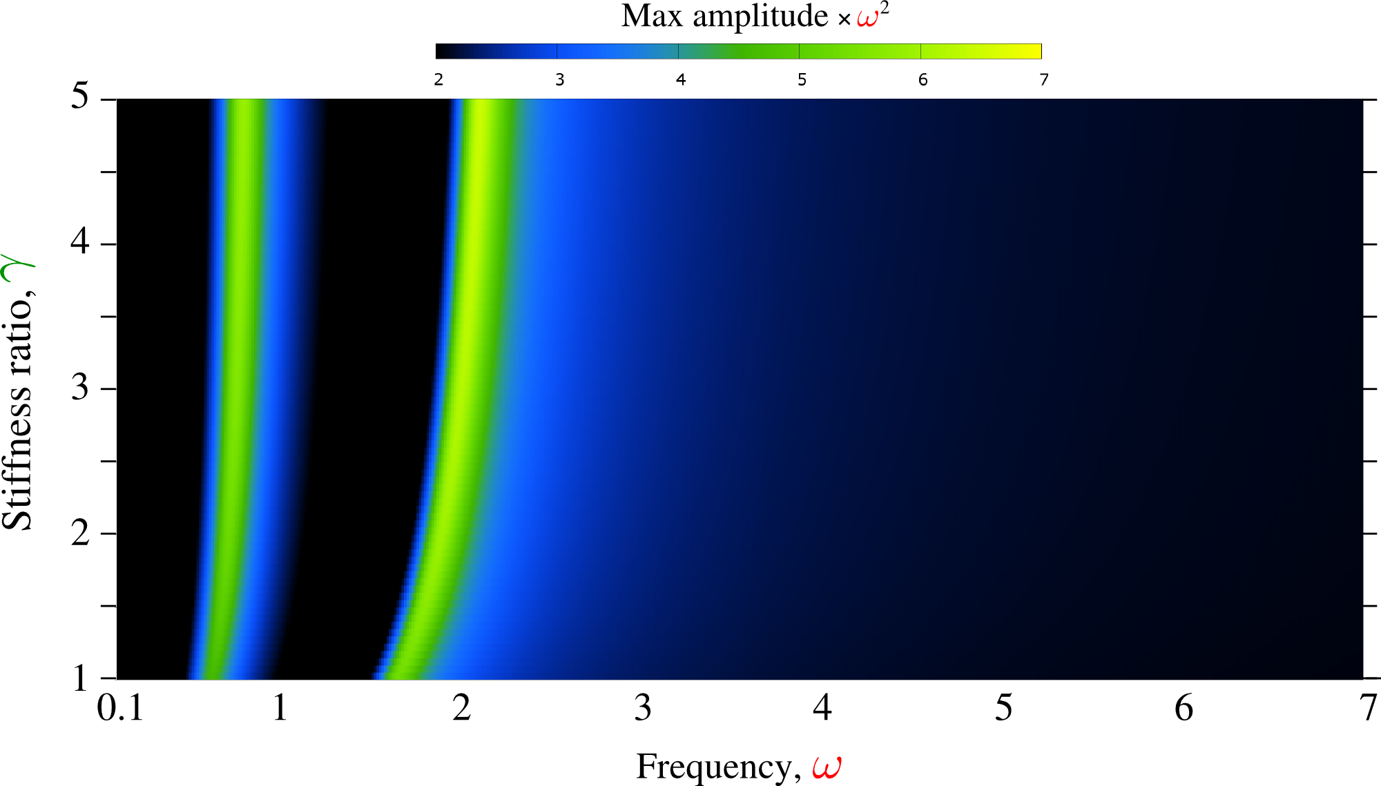
Frequency – elastic contrast – normalized maximal amplitude map for a symmetric -DOF material with the effective stiffness.
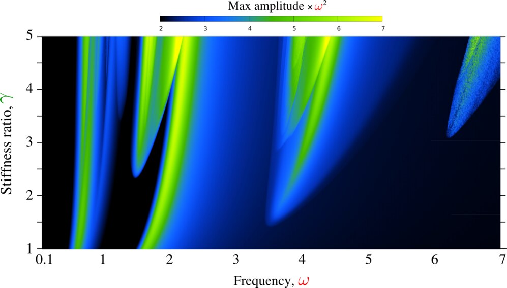
Frequency – elastic contrast – normalized maximal amplitude map for an asymmetric -DOF material.
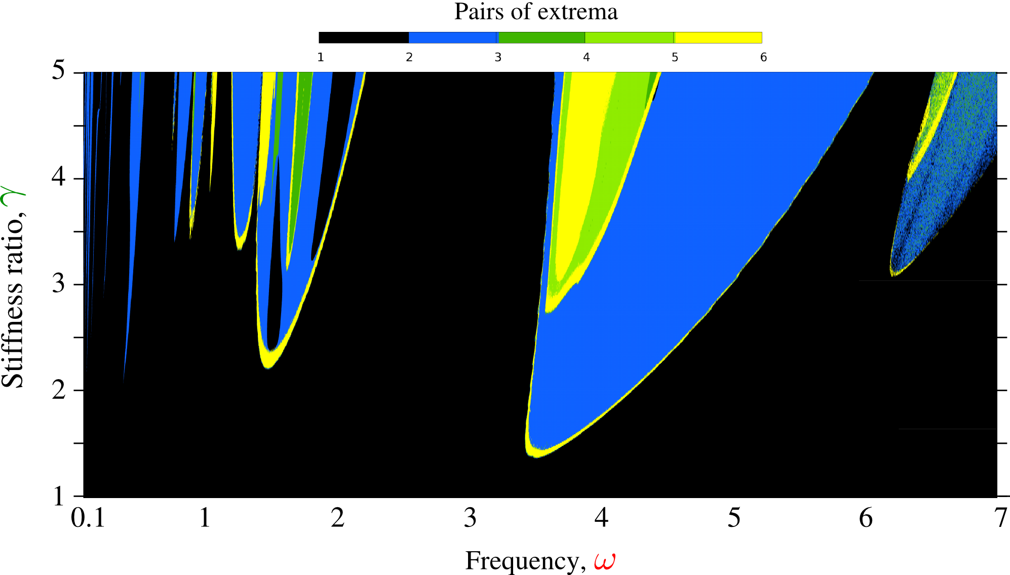
Frequency – elastic contrast – number of extrema in the amplitude for an asymmetric -DOF material.

Frequency – elastic contrast – number of Poincaré points per convergent cycle, equivalent to the number of periods, for an asymmetric -DOF material.
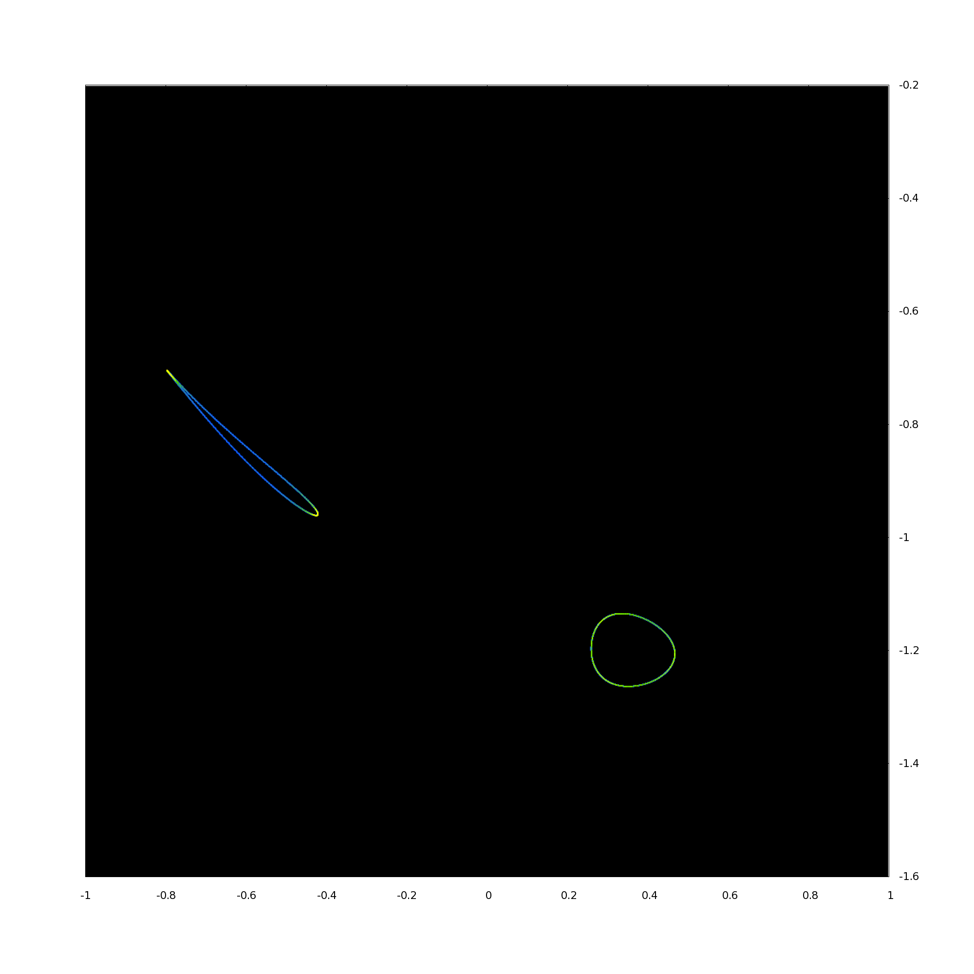
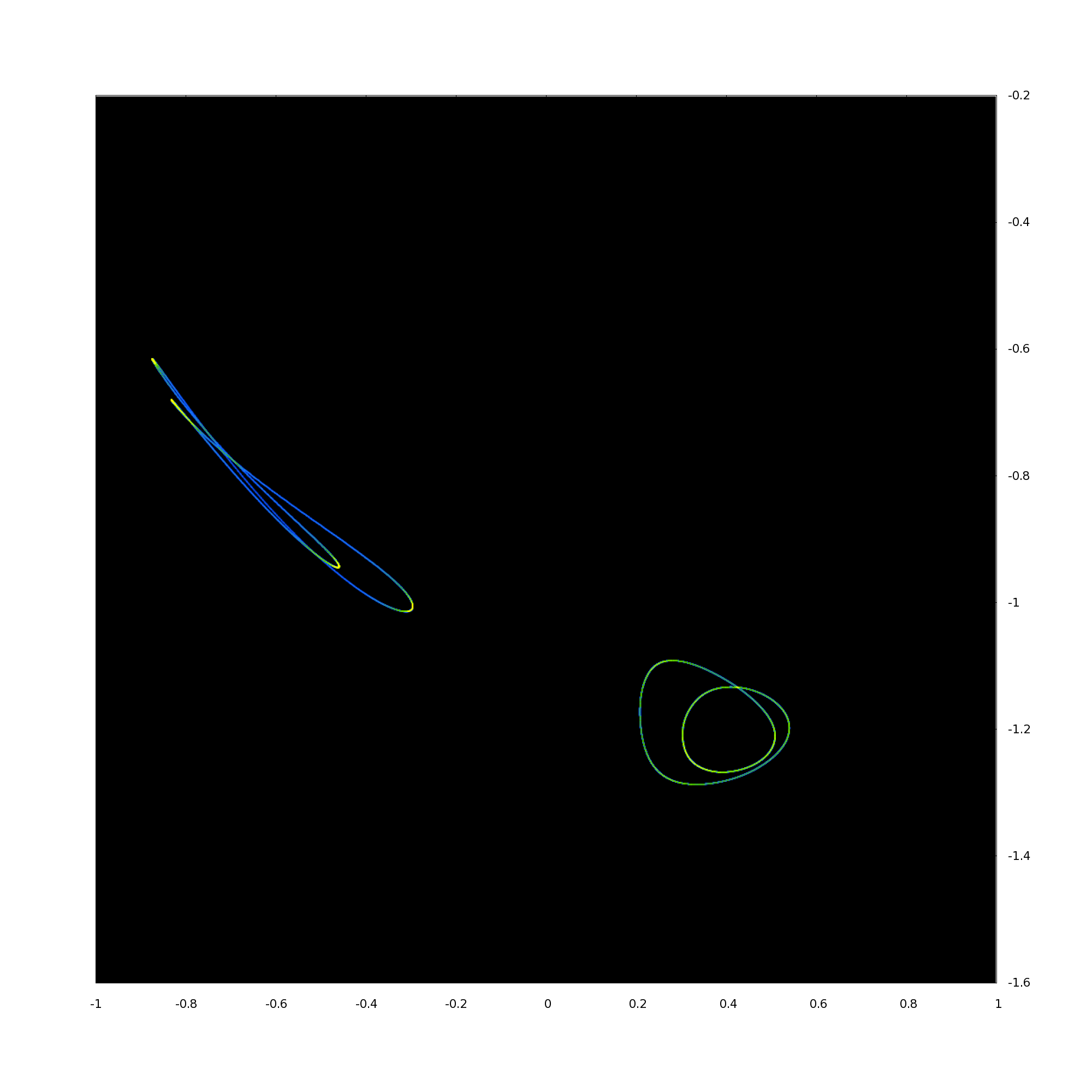
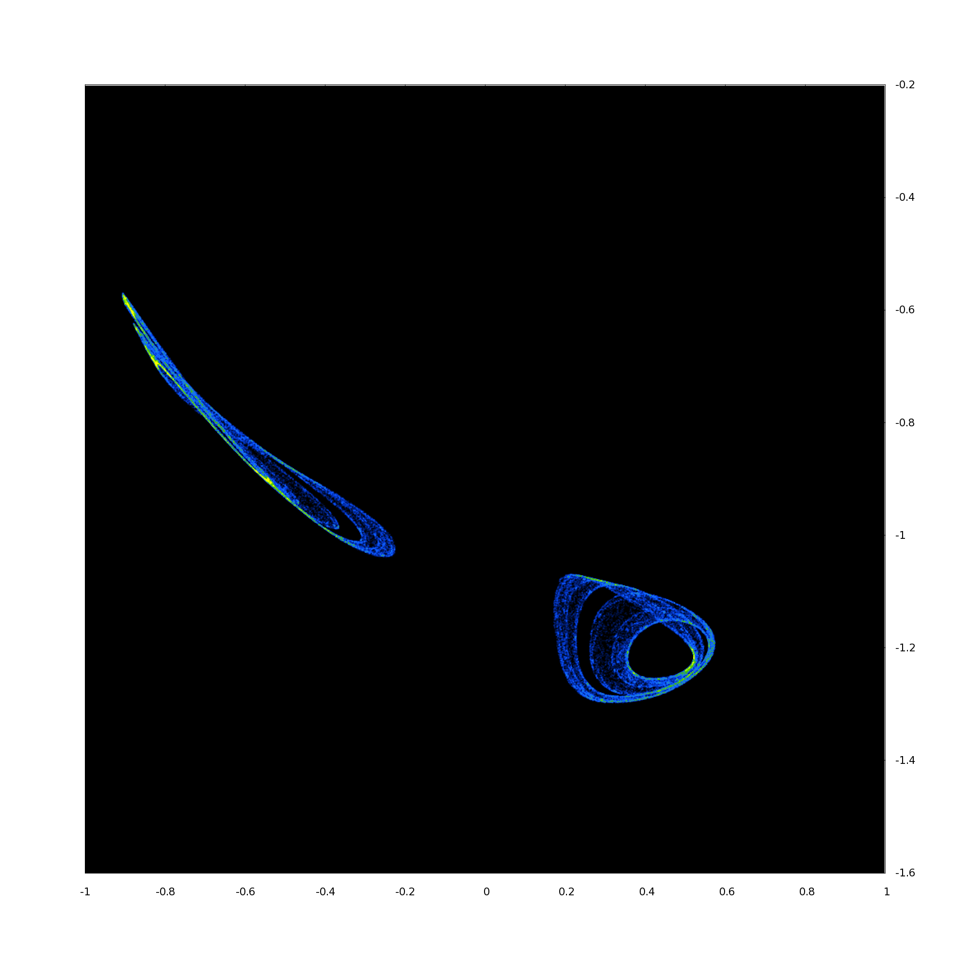
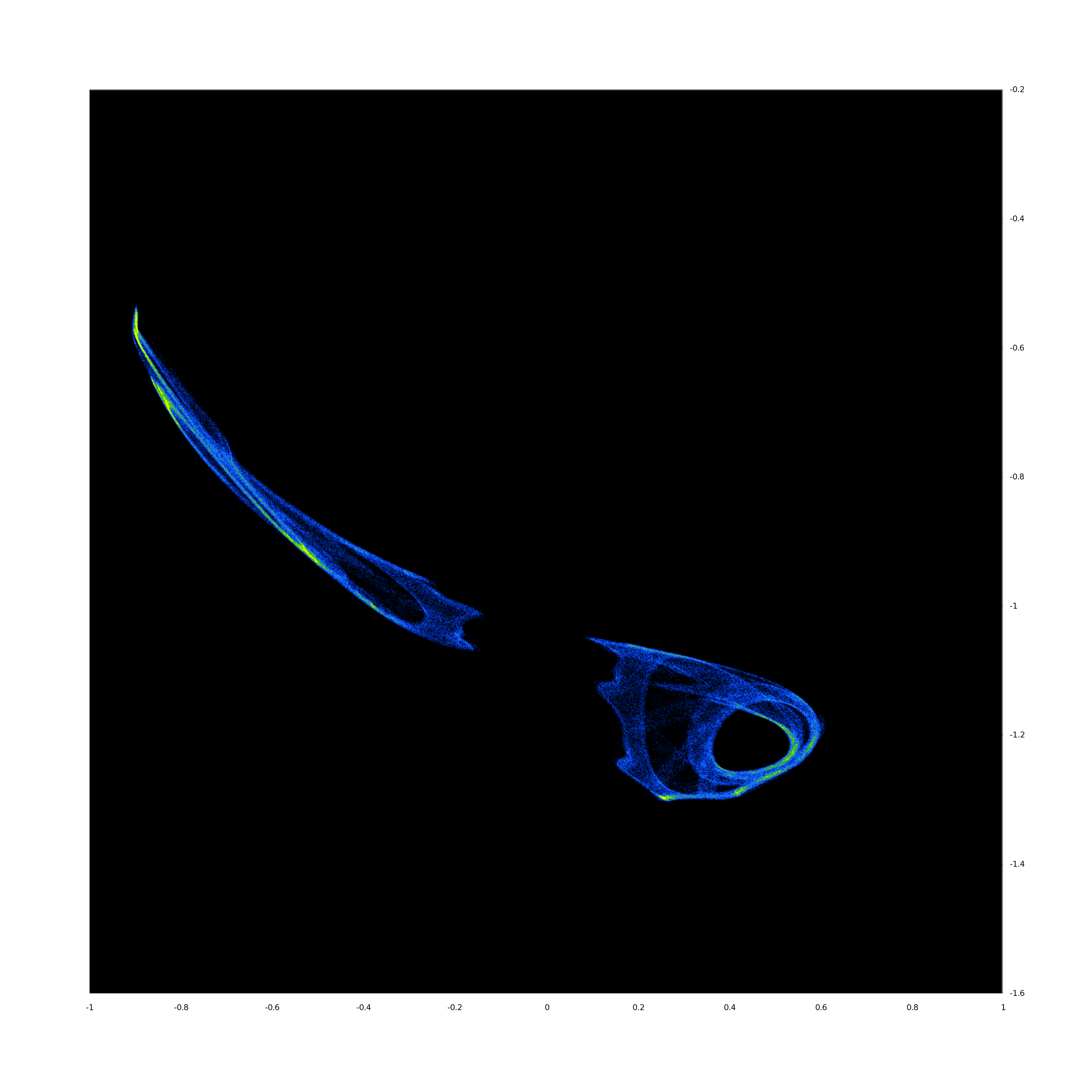
2D projection of 4D density of Poincaré points for , , from left to right – from Hopf trajectory (pseudo-periodic solution) to two-branch chaotic attractor (in terms of Poincaré points).
This study did not create new fundamental knowledge, it simply helped me to explore yet rather superficially and mainly “experimentally” the field of nonlinear dynamics. The fact that search for different dynamic regimes could be rather CPU-time consuming, we started to explore this non-linear dynamics using machine learning algorithms in the framework of 3 months internship of Yirun Zou. We started with simply trying to forecast the trajectory of one of the DOFs without the knowledge of the second DOF dynamics using a simple Multi-Layer Perceptron (MLP) neural network. Even though this attempt was quite successful, the true objective: predict the dynamic regime knowing the behavior over few first cycle appeared too ambitious and was not explored. An interesting result was that some trained MLPs could predict complex multiple-period cycles even though within their training data such cycles were absent.
Show animation.
3D projection of 4D Poincaré points of two different strange attractors, the color of points corresponds to the fourth missing degree of freedom.
📚 References
- Presentation “Nonlinear Oscillator: an attempt to predict butterfly effect by machine learning” with Yirun Zou [pdf]