🏠 Back to the Table of Contents
Research results
Glacial earthquakes: bedrock/glacier/iceberg/ocean interaction
Capsizing iceberg model
During the PhD project of Amandine Sergeant-Boy, we developed a simplified but still local fluid-solid interaction (FSI) model which apart from the hydrostatic pressure , could approximately evaluate and apply the hydrodynamic pressure within the finite strain finite element framework. The model of hydrodynamic pressure could take into account a background fluid velocity field and resulted in an acceptable approximating of the drag force Fig. 27. Thanks to this simplified model we could make a link between seismic signals and the source force induced by the iceberg-glacier interaction [81], see Fig. 28 and ultimately, Amandine Sergeant Boy on her own could carry out a global study on ice loss in Greenland using inverse analysis [82].
 Fig. 27
(Left) – drag factor (normalized drag force) for a solid of elliptic section found by our simplified geometrical drag model and compared with experimental results; (right) – pressure distribution obtained on an elliptic section using our simplified drag model and approximate experimental data for a circular section.
 Show animation.

An imaginary simulation of a drop of deformable solid into a super-dense but not too viscous liquid, its level is set to .
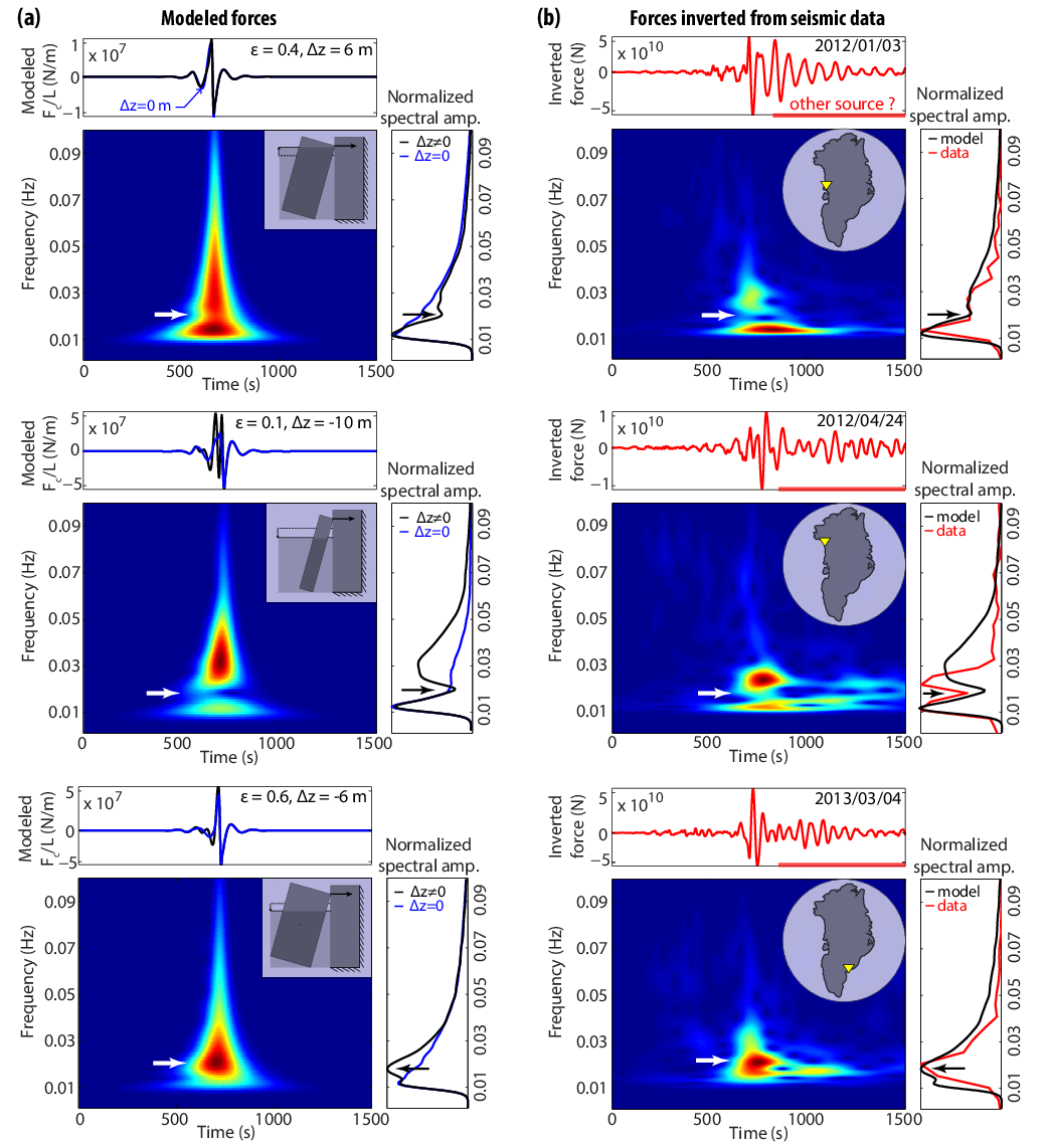 Fig. 28
Comparison of the forces (a) simulated with our simple iceberg-capsize model and (b) inverted from seismic data, both forces are filtered between 0.01 and 0.1 Hz, as well as the associated normalized spectrograms and power spectra. These simulated and inverted forces are for systems of non-equilibrium buoyancy (i.e., ). For the field data in Greenland (column (b)), locations of the calving events and GLISN stations used in the waveform inversion are indicated on inset maps by red stars and yellow triangles, respectively. The power spectra panels show the forces inverted from seismic data (red curves), modeled with either submarine or subaerial icebergs (black curves), and modeled with initially neutrally buoyant icebergs (blue curves). The comparison between models and data show that seismic data spectral peaks or gaps indicated by arrows can be explained by the initial buoyant state of the capsizing icebergs, especially when they are out of their flotation level when they calve and start to capsize [81].
Nevertheless, using a multi-DOF FE model for iceberg capsizes was an excessive solution, so we re-implemented the model for simple rigid solid dynamics with a leap-frog (Störmer-Verlet) integration in time and with the contact handled by the penalty method applied both to the penetration and to its rate to avoid spurious high frequency oscillations. In addition, this new model was complemented with a phenomenological added-masses and the moment of inertia using theoretical results of [83]. The resulting model was successfully compared with full scale 2D CFD simulations made by Patrick Queutey and Alban Leroyer using their powerful in-house ISIS-CFD software. However, this comparison was only possible in absence of contact, which cannot be handled by ISIS-CFD, i.e. we studied a rather artificial for the nature situation of an iceberg capsize in open ocean [84]. Nevertheless, this comparison allowed us to understand better the capsize dynamics, the effect of the scale and involved hydrodynamic forces and processes. The original drag model was slightly improved by adjusting better the added-mass and drag factors for rectangular icebergs of different aspect ratios. All results are compared with lab experiments in Fig. 29. Remarkably, our simple model can reproduce quite well kinematics of the iceberg capsize as well as the associated forces and moments.
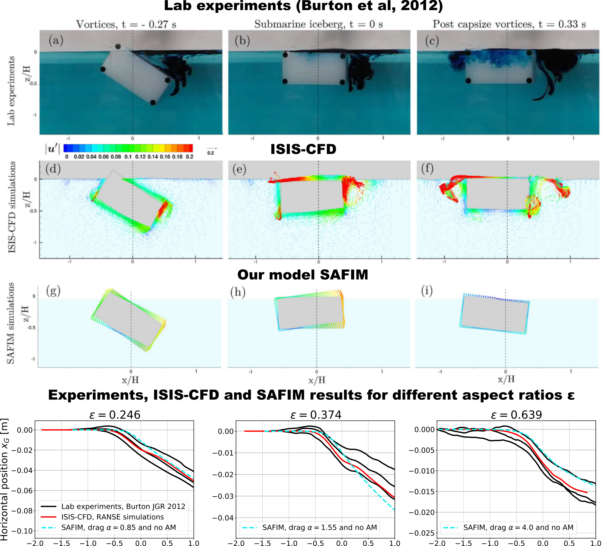 Fig. 29
Lab experiments from [85] compared with RANSE CFD simulations carried out by Patrick Queutey and Alban Leroyer using their powerful in-house ISIS-CFD software and compared with results of our Semi-Analytical Floating Iceberg Model (SAFIM). The lower model compares horizontal dynamics of the iceberg obtained numerically using our two models with experimental results.
📚 References
- [81] A. Sergeant, V.A. Yastrebov, A. Mangeney, O. Castelnau, J.P. Montagner, E. Stutzmann. “Numerical modeling of iceberg capsize responsible for glacial earthquakes”. Journal of Geophysical Research: Earth Surface, 123:3013-3033 (2018). [doi] [pdf]
- [82] A. Sergeant, A. Mangeney, V.A. Yastrebov, F. Walter, J.-P. Montagner, O. Castelnau, E. Stutzmann, P. Bonnet, V.J.L. Ralaiarisoa, S. Bevan, A. Luckman. “Monitoring Greenland ice-sheet buoyancy-driven calving discharge using glacial earthquakes”. Annals of Glaciology, 60(79):75-95 (2019). Open access. [doi] [pdf]
- [84] P. Bonnet, V.A. Yastrebov, P. Queutey, A. Leroyer, A. Mangeney, O. Castelnau, A. Sergeant, E. Stutzmann, J.-P. Montagner. "Modelling capsizing icebergs in the open ocean ". Geophysical Journal International, 223(2):1265-1287 (2020). [doi] [arXiv]
🏠 Back to the Table of Contents
Deformation of the glacier in response to iceberg capsize
Glacier flow combined with the sliding on the bedrock is slowed by frictional forces arising from volume dissipation in the visco-elasto-plastic ice as well as from melting and re-solidification of the ice in the rock/ice interface. The resulting friction law is viscous and is often referred to as Weertman law [86]. In our studies of glacial earthquakes in Greenland caused by capsize of unstable icebergs in contact with glaciers, we studied the visco-elasto-plastic deformation of the latter accompanied such events. At short time scales, the behavior of ice can be seen as elastic, and assuming that the glacier can be approximated by a bar interacting with the bedrock by Weertman’s law, we obtain, after some simplifications, a parabolic equation for the perturbation of displacement as a function of the axial force exerted by the iceberg . This equation is equivalent to the heat diffusion problem and takes the following form:
where the parameter (with being the parameter of Weertman’s law, Young’s modulus and the height of the glacier) is similar to the heat diffusivity. The solution of this equation can be found quite easily via Green’s functions to obtain the following form of the total displacement:
where is the density of the ice, is the acceleration of gravity and is the angle of the bedrock’s inclination. The numerical evolution of the integral in the Fourier series is quite heavy for an arbitrary form of the force . Therefore, we suggested an analytical form of this force which is in good agreement with CFD calculations of the iceberg/glacier front interaction. This form allows to simplify the evaluation of the mentioned integral. This simplification permits to rapidly evaluate the glacier’s dynamics in response to capsizing icebergs and thus permits to carry out a relatively broad parametric study for outlet glaciers in Greenland. In Fig. 30, the displacement of the typical glacier near the terminus caused by the capsize of a typical iceberg obtained by the integration of equation Eq. is shown. In addition, this study allowed us to make interesting connections between the behavior of ice as an elastic solid in the short term and its non-Newtonian flow in the longer term. The article is in preparation [87]. In parallel, a broad parametric finite element study with a 2D model was carried out both on model geometry with a constant slope and on a realistic geometry of Helheim glacier and its bedrock located in South-East Greenland. These simulations were carried out for different iceberg-capsize scenarios: top-out and bottom-out capsize which trigger different deformation regimes in the glacier, which could not been modeled with a simple 1D model described above. The work on related papers is in progress.
In order to model short-time-scale events, we need to know the initial state of the visco-elasto-plastic glacier which implies that we need to model its history taking into account its interaction with the ocean and the bedrock. Therefore, mainly in the framework of Pauline Bonnet PhD project, we studied a lot different models of marine sheets and carried out numerous numerical simulations, which we compared both with analytical solutions and numerical models of others.
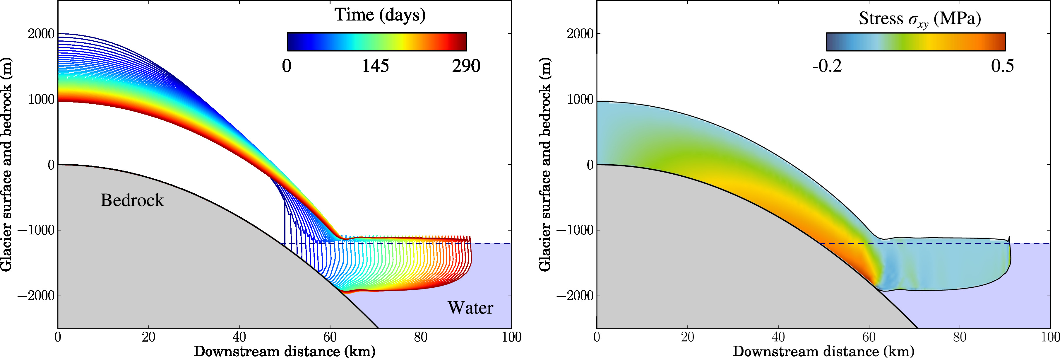
Fig. FE simulation of accelerated glacier flow into the ocean under Weertman friction law
 Version française (click to expand)
Le glissement des glaciers sur le lit rocheux est freiné par les efforts de frottement spécifique provenant de la dissipation volumique dans la glace visco-élasto-plastique ainsi que de la fusion et resolidification de la glace dans l’interface roche/glace. La loi de frottement résultante est de type visceux et elle est souvent reférencée comme une loi de Weertman [86]. Dans nos études des séismes glaciaires au Groenland provoqués par le retournement des icebergs instables en contact avec les glaciers, on a étudié également la déformation visco-élasto-plastique de ces derniers. Aux échelles de temps courts, le comportement de la glace peut être vu comme élastique, et dans l’hypothèse où le glacier peur être approximé par une bar intéragissant avec le lit rocheux par la loi de Weertman, on obtient, après quelques simplifications, une équation parabolique pour la perturbation du déplacement en fonction de la force exercée par l’iceberg . Cette équation est équivalente à celui du problème de diffusion de la chaleur et prend la forme suivante :
où le paramètre -avec le paramètre de la loi de Weertman, module de Young et la hauteur du glacier) est similaire à la diffusivité de la chaleur. La solution de cette équation peut être assez facilement trouvée via des fonctions de Green pour obtenir la forme suivante du déplacement totale:
où est la densité de la glace, est l’accélération de la pesanteur et est l’angle de l’inclinaison du lit rocheu. L’évolution numérique de l’integral dans le série de Fourier est assez lourde pour une quelconque forme de la force . Pour cela, nous avons trouvé une forme analytique de cette force qui est en accord avec des calculs CFD de l’interaction iceberg/front glacier et qui permet de simplifier l’évaluation de l’integrale mentionné. Cette simplification nous a permis de mieux comprendre la déformation du glacier en réponse au retournement de l’iceberg et faire l’analyse paramétrique pour des glaciers emissaire au Groenland. Sur Fig. 30, le déplacement du glacier type près du terminus provoqué par le vêlage d’un iceberg-type obtenu par l’integration de l’équation Eq. est repésenté. En outre cetté étude nous a permis a faire des liens intéressant entre le comportement de la glace en tant qu’un solide élastique à court terme et son écoulement non-Newtonien au temps plus longue. L’article est en phase de préparation [87].
 Fig. 30
Displacements in the glacier induced by its sliding on the constant slope superimposed with the displacement caused by the force excerted by capsize of an unstable iceberg.
Version française (click to expand)
Déplacements dans le glacier induits par son glissement sur la pente constante superposé avec le déplacement provoqué par le retournement d’une iceberg instable.
📚 References
- [87] Yastrebov, V.A., Bonnet, P., Mangeney, A. and Castelnau, O. ''Effect of iceberg’s capsize on the deformation of marine-terminating glaciers``, en préparation (2021). Draft of the article is available [encrypted pdf]