🏠 Back to the Table of Contents
Research results
Computational mechanics
Correction of discretization error in spectral BEM
The numerical study of the growth of the real contact area between rough surfaces under the action of the applied pressure requires a very fine discretization. First of all, a fairly wide spectrum of a surface should be represented. Additionally, the discretization must be sufficient to correctly solve the mechanical problem in classical terms of the mesh convergence. If the spectrum of the surface is well represented by the discretization, the error on the measurement of the contact area is concentrated exclusively at the edge of the contact zones (“spots” of contact) whose number can be very high depending on the size and the representativity of the surface, i.e. on the cutoff frequencies in the surface spectrum. The more representative the surface, the greater the number of contact zones, and therefore the greater the ratio between the perimeter and the area . For a grid of spacing , the relative error on the contact area is proportional to the ratio where is the exact solution obtained for [9]. Basically, this form of error suggests that the real solution lies between the value obtained in simulations and the same area without the area of its peripheral contact/non-contact transition zone of one-element thickness, i.e. . On the other hand, the value of is not easy to estimate. But we found a trick
Take a square and cut it in two part by a randomly oriented straight line; what will be in average the ratio between the area of the smallest part to the area of the square ? The answer is
If we use this number so that the contact area estimated by the numerical calculation is deprived of this fraction of its peripheral crown, and the latter is corrected by the transformation of the metric from (Manhattan metrics because we work on the square grid) to (Euclidean metrics) via a factor for shapes isotropic in average, we obtain a simple expression to estimate the contact area by minimizing the discretization error:
where is the total perimeter of the contact zones calculated on the square grid. This simple equation makes it possible to obtain the contact area very precisely even for very modest discretizations [88] (Fig. 31). As demonstrated in Section, this error compensation technique allowed us to go beyond the state of the art in the study of "rough contacts" and obtain new insights in the study of rough contact.
 Version française (click to expand)
L’étude numérique de l’évolution de l’aire de contact réelle entre des surfaces rugueuses sous l’action de la pression appliquée nécessite une discrétisation très fine. Il s’agit tout d’abord de représenter proprement un spectre assez large d’une surface mais par ailleurs la discrétisation doit être suffisante pour résoudre correctement le problème mécanique. Si le spectre de la surface est bien représenté par la discrétisation, l’erreur sur la mesure de l’aire de contact se localise sur le bord des zones et des “taches” de contact dont le nombre peut être très élevé en fonction de la coupure aux basses fréquences. Plus la surface est représentative, plus grand est le nombre de zones de contact, et donc plus grand est le ratio entre le périmètre et l’aire . Pour une grille d’espacement , l’erreur relative sur l’aire de contact est proportionnelle au ratio où est la solution exacte pour [9]. En gros, cette forme d’erreur suggère que la vraie solution se trouve entre la valeur obtenue par des simulations et la même aire privée de sa couronne périphérique d’épaisseur , i.e. .
Par contre la valeur de n’est pas facile à estimer. Nous avons donc trouvé une astuce\dots
Prenons un carré et coupons le en deux par une droite arbitraire ; quel sera le rapport entre l’aire du plus petit morceau et l’aire du carré en moyenne ? La réponse est
Si on utilise ce nombre de façon à ce que l’aire de contact estimée par le calcul numérique soit privée de cette fraction de sa couronne périphérique, et qu’à son tour celle-ci soit corrigée par la transformation de la métrique (celle de Manhattan comme on travaille sur la grille carrée) à via un facteur , nous obtenons une simple expression pour estimer l’aire de contact en minimisant l’erreur de discrétisation :
où est le périmètre total des zones de contact calculé sur la grille carrée. Cette équation simple permet d’obtenir l’aire de contact très précisément même pour de très modestes discrétisations [88] (Fig. 31). Comme cela va être démontré dans le résultat suivant, c’est cette technique de compensation d’erreur qui nous a permis d’aller au-delà de l’état de l’art dans l’étude des "contacts rugueux".
 Fig. 31
Convergence of the simulated contact area (a) without and (b) with discretization error compensation for a surface of size with the well-represented surface spectrum already with , i.e. the higher frequency cutoff is set to . It can be seen that with the compensation technique Eq. (C), the result almost does not depend on the discretization! The inset shows the distribution of the real contact area % found by the calculation.
Version française (click to expand)
Convergence de l’aire de contact mesurée (a) sans et (b) avec compensation d’erreur de discrétisation pour une surface de taille avec le spectre de surface bien représenté déjà avec . On constate qu’avec la technique de compensation Eq. (C), le résultat ne dépend pas de la discrétisation ! La figure en insertion montre la distribution de l’aire réelle de contact % trouvée par le calcul.
📚 References
- [9] V.A. Yastrebov, G. Anciaux, J.F. Molinari.
“From infinitesimal to full contact between rough surfaces: evolution of the contact area”.
International Journal of Solids and Structures, 52:83-102 (2015) [doi] [arXIv] [pdf] - [88] V.A. Yastrebov, G. Anciaux, J.F. Molinari.
“On the accurate computation of the true contact area in mechanical contact of random rough surfaces”.
Tribology International, 114:161-171 (2017) [doi] [arXIv] [pdf]
🏠 Back to the Table of Contents
MorteX method for tying, contact and wear
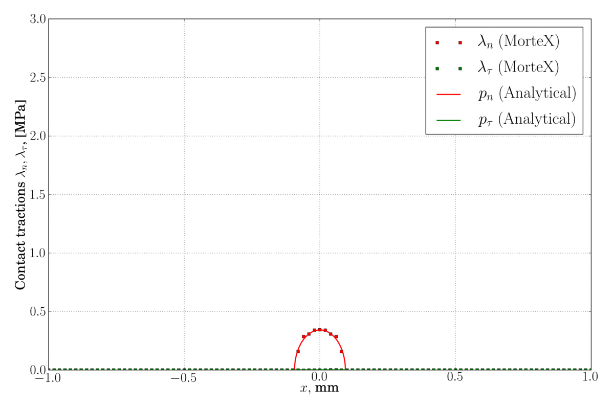
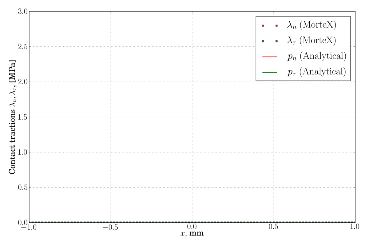
In PhD project of Basava Raju Akula (I could supervise this project in collaboration with Julien Vignollet (Safran tech) thanks to the trust of my thesis supervisor, Prof. Georges Cailletaud, who was the official supervisor), we have developed an original numerical method to deal with contact and sticking problems between virtual surfaces embedded in finite element mesh (cf. Fig. 32). The trick is to realize a combination of the X-FEM method [89] and the mortar method based on the monolithic augmented Lagrangian method; these two methods gave the name MorteX to our novel method. In addition to the purely technical difficulty related to the implementation of this coupling, there is a well-known theoretical obstacle in the world of extended finite elements: those are spurious oscillations that arise in the interface between bodies when the materials have a large difference in stiffness, or when the mesh densitis on tying sides contrast too much. We have proposed a coarse-grained Lagrange multiplier interpolation technique that avoids this problem [90]. The idea behind is to avoid over-constraint and adjust the number of available primal and dual DOFs in the interface. This technique has been successfully tested on classical patch tests as well as on the Eshelby inclusion problem; it has also proved useful for the classical Mortar method in the case of strong contrasts between the elastic properties or in presence of curvatures under-represented by FE discretization. Further the methodology was extended for contact problems between virtual surfaces [91].
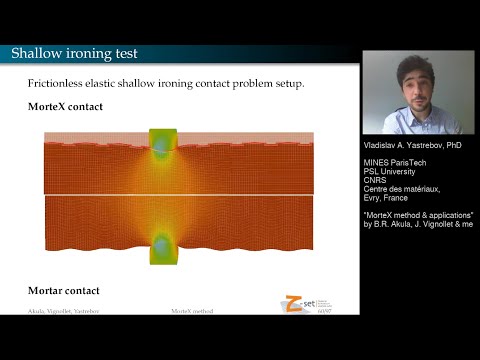
The MorteX method is especially adapted to treat wear problems [92]. In this case, the evolution of contact surfaces resulting from material removal due to wear is modeled as a virtual surface evolution that propagates within the existing mesh. The use of the MorteX method therefore eliminates the need for complex remeshing techniques. Currently, we are working on the optimization of the space of interpolation functions used for Lagrange multipliers. Our preliminary results suggest that the use of the so-called dual shape functions for Lagrange multipliers permits to avoid some inconsistencis in pressure interpolation near contact edges, which are inevitable within the standard interpolation scheme. See animations below.
 Show animation.
(left) – classical Legendre interpolation for Lagrange multipliers, some spurious oscillations are observed near the contact edge, (right) – discontinuous first-order dual shape function are used for Lagrange multipliers which considerably reduces these oscillations.
Version française (click to expand)
Dans le cadre de la thèse de Basava Raju Akula (c’est une thèse que j’ai dirigée grâce à la confiance qui m’a été accordé par mon directeur de thèse, Prof. Georges Cailletaud, qui en était le directeur officiel), nous avons développé une méthode numérique originale qui permet de traiter des problèmes de contact et de collage entre des surfaces virtuelles embarquées au sein du maillage élément finis (cf. Fig. 32). L’astuce consiste à réaliser une combinaison de la méthode X-FEM [89] et de la méthode de mortar basée sur le Lagrangien augmenté monolithique ; ces deux méthodes ont donné le nom MorteX à la nôtre. En plus de la difficulté purement technique liée à la mise en œuvre de ce couplage, il existe un obstacle théorique bien connu dans le monde des élément finis étendus : il s’agit d’oscillations parasites qui surgissent dans l’interface entre des corps lorsque les matériaux présentent une grande différence de propriétés élastiques, ou bien lorsque les densités de maillage sont très élevées. Nous avons proposé une technique d’interpolation des multiplicateurs de Lagrange à grains grossiers qui permet d’éviter ce problème [90].
Cette technique a été testée avec succès sur des “patch-tests” classiques ainsi que sur le problème d’inclusion d’Eshelby ; elle s"est également avérée utile pour la méthode Mortar classique dans le cas de forts contrastes entre les propriétés élastiques. Ensuite la méthodologie a été étendue pour des problèmes de contact entre des surfaces virtuelles [91].
La méthode MorteX est sutout adaptée pour traiter des problèmes d’usure [92]. Dans ce cas, l’évolution des surfaces de contact qui résulte de l’enlèvement de matière dû à l’usure est modélisée comme une évolution de surface virtuelle qui se propage au sein du maillage existant. L’utilisation de la méthode MorteX élimine donc le besoin de recourir aux techniques complexes de remaillage. Actuellement, nous travaillons sur l’optimisation de l’espace des fonctions d’interpolations utilisées pour les multiplicateurs de Lagrange.
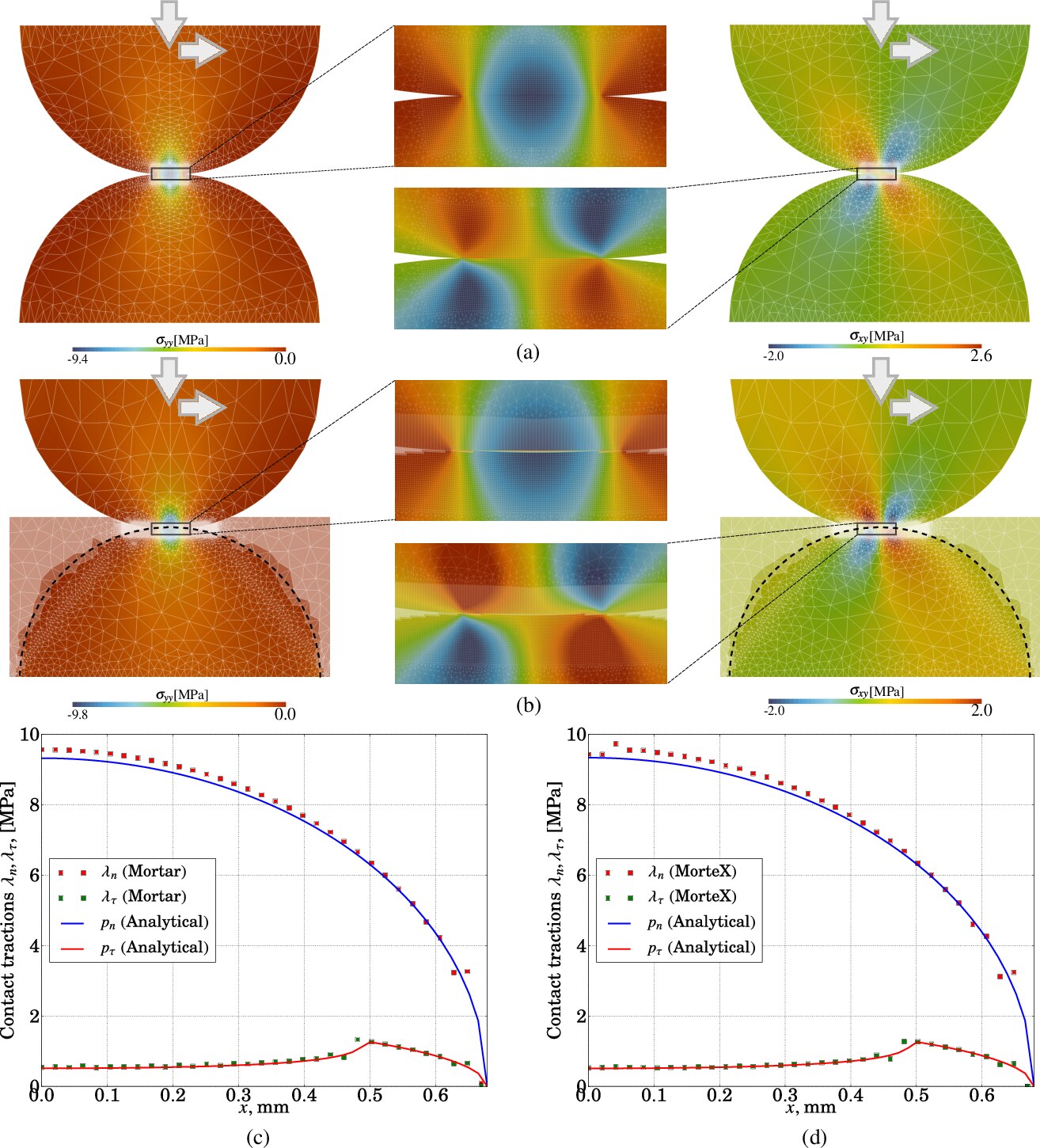 Fig. 32
Problem of the frictional contact between two identical cylinders. Comparison of (a) the classical mortar method (which uses a boundary-fitted discretization) and (b) the MorteX method in which one of the cylinders is defined by a virtual surface passing through the mesh of a rectangle; (c ) and (d) show normal and tangent traction distributions at the interface obtained by these two methods.
Version française (click to expand)
Problème du contact frottant entre deux cylindres. La comparaison de (a) la méthode classique de mortar avec la discrétisation conforme à la géométrie et (b) de la méthode MorteX dans laquelle un des cylindres est défini par un demi-cercle inseré dans le maillage d’un rectangle ; (c ) et (d) montrent des distributions de contraintes à l’interface obtenues par ces deux méthodes.
📚 References
- [90] B.R. Akula, J. Vignollet, V.A. Yastrebov (2019). “Stabilized MorteX method for mesh tying along embedded interfaces”. Preprint is available [arXiv] [pdf]
- [91] B.R. Akula, J. Vignollet, V.A. Yastrebov (2019). “MorteX method for contact along real and embedded surfaces: coupling X-FEM with the Mortar method”. Preprint is available [arXiv] [pdf]
- [93] B.R. Akula “Extended mortar method for contact and mesh-tying applications”. PhD thesis defended on the 4th of February 2019 at Ecole des Mines de Paris, Paris, France. Supervisors: G. Cailletaud, J. Vignollet, V.A. Yastrebov. PhD committee: M.C. Baietto (president), A. Popp (reviewer), F. Lebon (reviewer), N. Moës, V. Chiaruttini. [HAL]
- [92] B.R. Akula, J. Vignollet, V.A. Yastrebov (2020). “MorteX method for the simulation of wear” submitted. Draft is available [encrypted pdf]
- Extended presentation “The MorteX method and its applications”, World Congress on Computational Mechanics, Paris (virtually), France. January 2021 [youtube]
🏠 Back to the Table of Contents
Computational framework for coupled thin flow in contact interfaces
In addition to the study of dry contact, we studied various effects resulting from the presence of a fluid in the contact interface. These studies were carried out in the context of normal contact in the absence of any effort or tangential movement. This problem is relevant for several applications, among others: static sealing of systems, lubrication in hot/cold-rolling and other types of metal forming, hydrogeology, extraction of shale oil and gas, tire/road contact in wet conditions, and a large number of biomechanical contact problems in presence of fluid.
As part of the thesis of Andrei Shvarts (I was allowed to supervise this thesis thanks to the trust that was granted to me by my thesis director, Prof. Georges Cailletaud, who was the official director), we built a coherent and monolithic finite element framework to address problems of viscous saturated flow in contact interfaces between solids [94]. This problem is not new, but we have been able to build an original framework which is more complete than existing ones. The novelty consists in a careful treatment of “lakes” of trapped fluid, i.e. the fluid regions completely surrounded by the contact areas. This mechanism was incorporated into the monolithic finite element framework which solves the global non-linear system for (1) the displacement field in the solid, (2) the pressure field in the thin film of fluid governed by the Reynold equation, (3) the field of Lagrange multipliers necessary to ensure the conditions of Hertz-Signorini-Moreau contact, and finally (4) the pressures in the trapped fluids obeying a non-linear behavior. In this framework, the Reynolds equation is solved on the updated geometry, and the fluid in the trapped zones and in the flow exerts surface forces on the solid Fig. 33. What is important is that we have used a model of compressibility of the fluid in the trapped zones which is sufficiently representative of the relevant physics of the phenomenon: the modulus of compressibility increases in an affine manner with the pressure in the fluid (liquid). This numerical framework allowed us to explore the system behavior under the strong coupling between solid and fluid equations, and to deduce some new theoretical results, for example, an empirical law for non-local permeability.
Version française (click to expand)
En complément de l’étude du contact sec, nous avons travaillé sur l’effet de la présence d’un fluide dans l’interface de contact.
Cette étude est menée toujours dans le contexte du contact sous un effort normal, en absence de tout effort ou mouvement tangentiel.
Ce problème est pertinent pour plusieurs applications, entre autres : l’étanchéité des systèmes, la lubrification dy laminage et formage, l’hydrogéologie, l’extraction d’hydrocarbures de couches de schiste, le contact pneu/chaussée en conditions humides, et un grand nombre de problèmes de contact anatomiques en présence de fluide.
Dans le cadre de la thèse d’Andrei Shvarts (c’est une thèse que j’ai dirigée grâce à la confiance qui m’a été accordéee par mon directeur de thèse, Prof. Georges Cailletaud, qui était le directeur officiel), nous avons construit un cadre élément-finis cohérent et monolithique pour aborder des problèmes d’écoulement visqueux et saturé dans l’interface entre des solides en présence du contact [94]. Ce problème n’est pas nouveau, mais nous avons pu construire un cadre qui nous semble plus complet que ceux qui existaient auparavant. La nouveauté consiste en un traitement soigneux des îlots (ou plutôt des flaques) de fluide piégé, i.e. le fluide complètement entouré par les zones de contact. Ce traitement a été intégré dans le cadre monolithique élément finis qui résout le système global non-linéaire pour (1) le champ de déplacements dans le solide, (2) le champ de pression dans la couche mince de fluide gouverné par l’équation de Reynolds, et (3) le champ de multiplicateurs de Lagrange nécessaire pour assurer les conditions de contact de Hertz-Signorini-Moreau, et enfin (4) les pressions dans le fluide piégé à comportement non-linéaire. Dans ce cadre, l’équation de Reynolds est résolue sur la géométrie actualisée, et le fluide dans les zones piégées et dans l’écoulement exerce des efforts surfaciques sur le solide Fig. 33. Ce qui est important, c’est que nous avons utilisé un modèle de compressibilité du fluide dans les zones piégées qui est suffisamment représentatif de la physique du phénomène : le module de compressibilité augmente d’une manière affine avec la pression dans le fluide (liquide). Ce cadre numérique nous a permis d’explorer le comportement local fortement couplé entre solide et fluide, et de déduire quelques nouveaux résultats théoriques notamment sur la perméabilité non-locale.
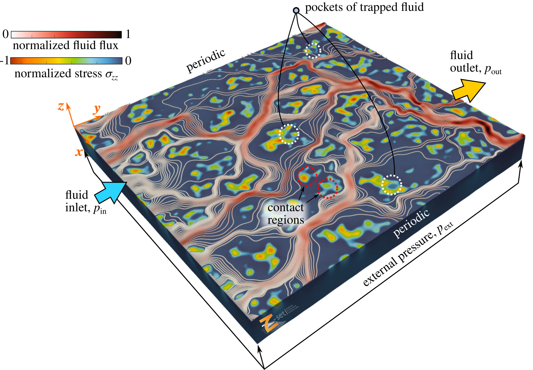 Fig. 33 Strongly coupled simulation of thin flow in contact interface (couloured spots represents contact areas, flow lines represent direction and intensity of the main flux channels, lakes of trapped fluid are highlighted).
Version française (click to expand)
Simulation d’écoulement dans l’interface de contact : couplage fort
Animations of a flow simulation through the contact interface of (left) an atoll-like structure under increasing pressure and (right) a rough surface in contact.
📚 References
- [41] A.G. Shvarts, V.A. Yastrebov. “Fluid flow across a wavy channel brought in contact”. Tribology International, 126:116-126 (2018). [doi] [arXiv] [pdf]
- [94] A.G. Shvarts, J. Vignollet, V.A. Yastrebov.
“Computational framework for monolithic coupling for thin fluid flow in contact interfaces”.
Computer Methods in Applied Mechanics and Engineering, 379:113738 (2021) [doi] [arXiv] [pdf] - Supplementary videos [zenodo]
- [26] A.G. Shvarts. “Coupling mechanical frictional contact with interfacial fluid flow at small and large scales” (2019). PhD thesis defended on March 20, 2019 at École des Mines de Paris in presence of the jury Res. Dir. D. Lasseux, Prof. M. Paggi, Prof. S. Stupkiewicz, Prof. J.A. Greenwood, Assist. Prof. V. Rey, Assist. Prof. N. Moulin, Prof. G. Cailletaud, Dr. J. Vignollet, Dr. V.A. Yastrebov. This PhD thesis was awarded by a 🏆 CSMA award for one of two best theses in computational mechanics and by 🏆 Hirn award for the best thesis in tribology.
[HAL] [pdf]